This is the first installment of the “Complexity Series”, where I endeavor to argue that there are certain classes of problems (simple arithmetic being one of them) that Transformer architectures will never be able to solve.
To get started, I want to do a deep dive on known algorithms that Transformers have used to perform simple arithmetic. There are thus far a few algorithms that researchers have discovered are being implicitly implemented by LLMs to be able to perform simple arithmetic. They include:
- The “Clock” algorithm (Kantamneni and Tegmark)
- Bag of Heuristics (Nikankin et. al, Anthropic)
- Digit-wise and Carry-over Circuits (Quirke and Barez)
The first method is the “Clock” method. The Kantamneni paper has a number of shortcomings that severely kneecap its ability to explain mechanistically how the various components that they discover in the model (chiefly, the “number helix”) are used to perform the end computation of $a + b$, but does explicitly mention how they discovered the number helix (or, if you remove the linear component from the helix, it becomes a number circle). This makes it somewhat of a mimicry of a preceding paper - Progress Measures For Grokking Via Mechanistic Interpretability - in terms of its contribution, except that it focuses on a cousin problem (general arithemtic and not modulo arithmetic), and on a more complex model.
Progress Measures For Grokking Via Mechanistic Interpretability (henceforth referred to as the Nanda paper) is the original paper which introduces the Clock algorithm. It focuses on modulo arithmetic ($(a + b) \mod P = ?$) and uses a much simpler model (1 layer Transformer with no layer normalization and effectively no positional encodings as they turned out to be irrelevant). The Nanda paper also suffers from the same limitations that kneecap its ability to explain mechanistically how the number circle is used. Yes, they prove the existence of periodic components (number circles) through Fourier Decompositions, and are able to argue Modus-Tollens style (by ablating these periodic components out and seeing model performance drop completely to chance) that these periodic components are indeed crucial to the computation of modulo arithmetic, but this isn’t quite sufficient to gain a deep, intuitive, and mechanistic understanding of just how the number circles are formed and used.
It is this deep, intuitive, and mechanistic understanding of how the circles are formed and used that allows us to really understand this flavor of computational circuitry, and to even begin to make arguments (even if just hand-wavy) of the robustness of such circuitry, its failure modes, and how to improve on them. For this reason, this blogpost will be all about really diving deep into the circuitry of modulo arithmetic, using the same problem setup and model as the Nanda paper, but going far deeper and more explicit than the paper does.
1. Objective
The idea of the Clock algorithm is this: a 1-layer transformer model trained to do modulo arithmetic learns how to encode numbers not as a number line in its weight space, but as a number circle (in fact, multiple number circles). This algorithm is interesting because it appeals to the intuitive idea that written numbers that we humans use have periodic patterns (e.g. digits go from 0 to 9 before wrapping around and repeating), and so, representing numbers in a cyclic mechanism could allow models to accurately perform simple or modulo addition. In the case of modulo arithmetic, the mental image this evokes is simple and beautiful; e.g. LLMs represent numbers on a circle much like a clock, and doing (10 + 6) % 12 = 4, much like how “10 o’clock + 6 hours = 4 o’clock.”
As mentioned, in both the Kantamneni and Nanda papers, the authors demonstrate proof that this circular representation of numbers actually exist (via Fourier Decompositions of embedding weights) in models specifically trained to perform simple / modulo arithmetic. Both papers also go on to use ablations, activation patching, and other methods to identify parts of the model that MUST be involved in the arithmetic computation, and essentially argue, modus tollens, that these circular components (and also select MLP neurons in the Kantamneni paper) are crucial to the computation. The result they present is simply that these components are used, and not how. That is to say, they still don’t quite fully paint a picture of how the model is “reading out” the answer, or how the clock is actually transforming / rotating and used in the various parts of the model.
For example, they establish that the columns of the embedding matrix $W_E$ (i.e. dictionary matrix) contain circular structures - that is to say, both a and b in “$(a + b) \mod P = ?$” will take on some point in these circles. However, how does the attention block transform and mix their representations? Attention is very obviously a non-linear transformation - how is it that we still see circles (spoiler: we do) after going through the attention block? How do these patterns change when we vary a and b? What computation is the MLP (specifically, the $\text{ReLU}$ non-linearity) block conceptually doing and how does that help the read-out function that is performed by the un-embedding matrix $W_U$?
I think that researchers (myself included) who intend to build on computational circuitry discovery with respect to interesting structures in embedding weights (circles in this case) should feel very uneasy about the lack of clarity here; how will you make predictions on things like effects of architectural changes or sufficiency conditions to be able to solve a class of problems if you cannot write a mechanistic description of existing “known” algorithms? Hence, this post aims to re-construct the Modulo Arithmetic Paper with special focus on:
✅ = Replication. ⭐ = Novel Contribution.
- ✅ Confirming that $W_E$, $W_L = W_U W_\text{down}$ (per Nanda; I go on to illustrate actually that only $W_U$, and not $W_\text{down}$, has to have a circular structures) contain circles and visualizing them
- ⭐ Investigating and illustrating what the attention block (both on a per-head basis and on an aggregate basis) is doing to the original circles in $W_E$
- ⭐ Investigating what the MLP block is doing to these circles
- ⭐ Illustrating the rotation of the circles and explaining how that is achieved
- ⭐ Demonstrate alignment between rows of $W_U$ (the unembedding matrix; refer to architecture diagram below) and appropriate embeddings in the circle to show how read-out of correct answer is done.
- ⭐ Arguing sufficiency conditions for Clock Algorithm to work (how many circles, circle frequency relationships)
2. Model Task
To restate the paper’s model task, a simple 1-layer Transformer is trained to finish the statement: {a} + {b} = where a and b are numbers $\in [1, P]$, where $P$ is some prime, in this case $113$, and the answer is the mathematical answer to $a + b \mod P$.
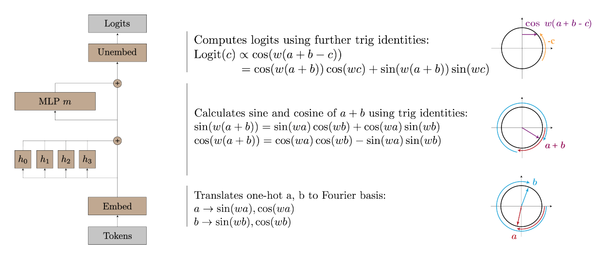 Model Architecture and Illustration of Periodic Representation
2.1. Exact Inputs and Outputs
The model is trained on simple input triplets of tokens: (token_A, token_B, token_C), where token_C is ALWAYS token index 113, which represents the = sign. token_A and token_B will simply be the index of the number they represent, i.e. token index 0 represents the number 0, token 42 represents the token 42, and so on.
Sometimes I’ll refer to
tripletsaspairssince onlytoken_Aandtoken_Bare meaningfully variable.
The target label is calculated by (token_A + token B) % P, where P = 113. This will be matched against the argmax of the raw outputs of the model, which are logits of shape (d_vocab,), where d_vocab = P + 1 = 114 (remember the extra token due to the = token). The loss is hence CrossEntropyLoss.
2.2. Train and Test Data
Just like in the paper, we generate all (token_A, token_B) pairs and randomly obtain a 30% split for the train set and use the remainder as the test set.
3. Architecture
This image fully illustrates the architecture of the 1-layer transformer that we’ll use to reproduce this paper:
 Architecture of 1-Layer Transformer We Use to Reproduce Paper
Things to note:
- There is no layer norm
- There are no positional embeddings
- MLP activation function shall be $\text{ReLU}$
Both the layer norm and positional embeddings intuitively don’t play a crucial role in this narrow task, and were confirmed to be irrelevant in the paper.
3.1. Equations
Because this blogpost is long and refers to the many parts of the model, I will write out all the equations here. The inputs are simply token indices (e.g. the inputs for the example “$(0 + 14) \mod P = ?$” are (0, 14, 113). All equations here are for 1 particular token (token position $t$). These are all just rather standard transformer components and I would just focus on the terminology of the subspaces (e.g. $z$ refers to head-wise attention output spaces, $o$ refers to aggregate attention output space, ‘MLP activation’ refers to post-$\text{ReLU}$ vectors, and so on).
Embedding Block
1
x_t = W_E[:, token_index_for_token_t]
Attention Block
\[\begin{align*} k_\text{t, head i} & = W_{K \text{, head i }} x_t \\ q_\text{t, head i} & = W_{Q \text{, head i }} x_t \\ v_\text{t, head i} & = W_{V \text{, head i }} x_t \\ \\ \text{attn vector}_\text{t, head i} &= \frac{1}{\sqrt{d_\text{model}}} \begin{bmatrix} q_\text{t, head i} \cdot k_\text{0, head i} \\ \vdots \\ q_\text{t, head i} \cdot k_\text{t, head i} \end{bmatrix} \\ \text{attn scores / activations /}a_\text{t, head i} &= \text{softmax}(\text{attn vector}) \\ \\ z_\text{t, head i} & = a_\text{t, head i} \cdot \begin{bmatrix} v_\text{0, head i} \\ \vdots \\ v_\text{t, head i} \end{bmatrix} \\ \\ o_\text{t} & = W_O \begin{bmatrix} v_\text{t, head 0} \\ \vdots \\ v_\text{t, head 3} \\ \end{bmatrix} \end{align*}\]MLP Block
\[\begin{align*} \text{MLP input}_t & = o_\text{t} + x_t \\ \text{MLP pre-ReLU vector}_t & = W_\text{up } \text{MLP input}_t + b_\text{up} \\ \text{MLP activation}_t & = \text{ReLU}(\text{MLP pre-ReLU vector}_t) \\ \text{MLP out}_t & = W_\text{down} \text{MLP activation}_t \end{align*}\]Unembedding Block
\[\begin{align*} \text{logits}_t = W_U (\text{MLP out}_t + \text{MLP input}_t) \end{align*}\]4. Achieving 0 Test Loss
The first step is obviously to make the model learn (grok) modulo arithmetic. We know that this is achieved when the model achieves 0 test loss, which it does:
Notice that the test accuracy hits 100% at about 4,000 epochs, but just for good measure, I let the model train till 10,000 epochs. This is just in case the regularization (AdamW) is still hard at work shrinking irrelevant weights (or weights dedicated only to memorization and not generalization) to 0; as you can see, the sum of squares of the W_E weight matrix still continues to decrease till about 6,000 steps.
5. Inspecting Periodicity
Before we can even try to tackle the objectives of this blog post, the next step is to confirm that there is some periodic mechanism in the weights, which we do by performing a Discrete Fourier Transform (DFT) on W_E, just as the authors have done. Also, because the authors hand-implemented DFT and left out some code, I’m including my code here for completeness.
Code of DFT
def inspect_periodic_nature(model: Transformer, do_DFT_by_hand: bool = False):
    """
    We want to see high-magnitude fourier components for:
    1.  W_E
    2.  W_L = W_U @ W_out
    """
    W_E = model.embed.W_E.detach().cpu()                    # shape (d_model, d_vocab)
    W_E = W_E[:,:-1]                                        # shape (d_model, P)
    # We expect periodicity over the vocab dimension.
    d_model, P = W_E.shape

    fig, ax = plt.subplots(1, 1, figsize=(12, 4))
    cmap = plt.get_cmap('coolwarm', 7)

    if do_DFT_by_hand:
        fourier_basis = []

        # start with the DC freq
        fourier_basis.append(torch.ones(P) / np.sqrt(P))

        # All the pairs of sin cos
        for i in range(1, P // 2 + 1):
            fourier_basis.append(torch.cos(2 * torch.pi * torch.arange(P) * i/P))
            fourier_basis.append(torch.sin(2 * torch.pi * torch.arange(P) * i/P))
            fourier_basis[-2] /= fourier_basis[-2].norm()
            fourier_basis[-1] /= fourier_basis[-1].norm()

        fourier_basis = torch.stack(fourier_basis, dim=0)   # Shape (P, P), waves going along dim 1

        fourier_coeffs = W_E @ fourier_basis.T
        fourier_coeff_norms = fourier_coeffs.norm(dim=0)

        x_axis = np.linspace(1, P, P)
        x_ticks = [i for i in range(0, P, 10)]
        x_tick_labels = [i // 2 for i in range(0, P, 10)]

        colors = [cmap(2) if i % 2 == 0 else cmap(5) for i in range(P)]
        ax.bar(x_axis, fourier_coeff_norms, width=0.6, color=colors)
        ax.set_xticks(x_ticks)
        ax.set_xticklabels(x_tick_labels)
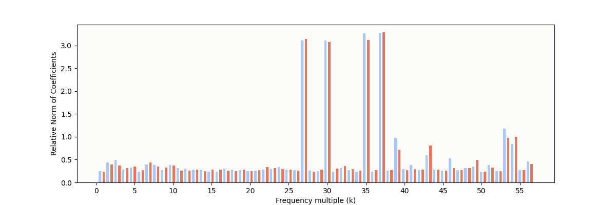 My W_E Fourier Coefficient Norms
The expected characteristic is definitely present: some frequencies have very high relative norms, indicating some sparse periodic structure. However, it’s still noticeably different from the result reported in The Modulo Arithmetic Paper:
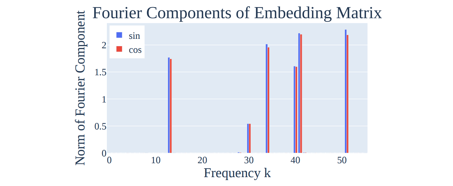 Their W_E Fourier Coefficient Norms
In particular, these are the differences I note:
- The original paper’s “inactive”
W_Ecoefficient norms are very small (basically 0) - The original paper’s “active”
W_Efrequencies are very clear and clean, whereas I only managed to produce 4 clean pairs in this run, with a few other frequencies being somewhat in-between in norm. - The frequencies that are “active” are different from the set of 5 that they cited in the paper.
5.1. More Weight Decay Time = Cleaner, Fewer Circles
My hunch for the first two points above is that the weight decay works over the training process to slowly pare away frequencies that the model can afford to do without, and that I simply haven’t allowed the model enough weight decay time to do that. To support this claim, I did another training run with fewer (5,000) and more (20,000) epochs, below. As for point (3), that is not of any concern as the model doesn’t have to learn any specific set of frequencies, so long as those frequencies are useful (what is “useful” will be explained all the way at the end, and it will make a lot of sense).
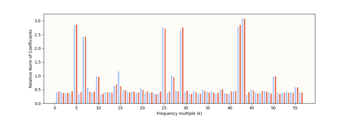
5,000 Epochs
 My W_E Fourier Coefficient Norms (5,000 epochs)
Notice I have even more “active” frequencies, that the model has ostensibly not “cleaned up.”
20,000 epochs:
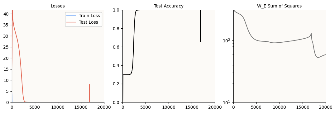 Training Metrics (20,000 epochs)
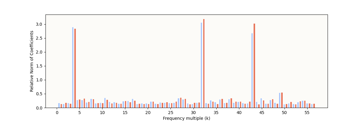 My W_E Fourier Coefficient Norms (20,000 epochs)
You can see that there are fewer but cleaner frequency norm spikes now.
One of my initial questions when reading the original paper was - why 5 circles? It seems intuitive that you only need 1 circle - why did the model settle on 5? I guess we now know that multiple local periodic structures form simultaneously, and the model eventually prefers the higher-signal periodic structures and pares away the redundant / lower signal structures; 5 was just an arbitrary number that the original authors happened to arrive at. As it turns out, the minimum number of circles is also 2 and not 1, for reasons that will become clear at the end.
5.2. Looking at the Circular Embeddings (W_E Columns)
Now that we have a grokked model to work with (I’m just going to use the 20,000 epochs one), we can attempt to see if we can actually visualize these embeddings.
Given that:
- We know there’s some periodic structure along the
d_vocabdimension ofW_E - We know what the Fourier Coefficients for each frequency (
k) are
Let’s try to visualize the embeddings in 2 chosen dimensions to see if the embeddings are indeed spherical. How may we choose the 2 dimensions? Well, if we computed our Fourier Coefficients Norms as such:
1
2
fourier_coeffs = W_E @ fourier_basis.T              # shape (d_model, P)
fourier_coeff_norms = fourier_coeffs.norm(dim=0)    # shape (P,)
Then, to visualize the circular structure for k = 4, we would simply take fourier_coeffs[:, [1 + 2 * (k - 1), 2 + 2 * (k - 1)]] (i.e. the columns that correspond to the sin and cos d_model-dimensional coefficients for k = 4) as the 2 basis vectors. From now on, we’ll call this the Fourier-Inferred 2D Basis (k Hz Circle) or Fourier-Inferred 2D Subspace (k Hz Circle). Then, we would simply project the 113 W_E vectors onto these 2 basis vectors (normalized) and see what we get.
We get the circles, as expected:
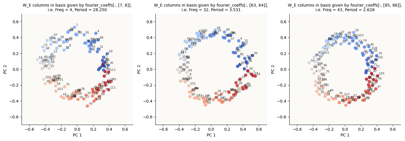 W_E columns in Fourier Coefficient Basis for k in {4, 32, 43} (20,000 epochs)
In case you were wondering how I color-coded the points to get such a continuous spectrum, I simply did this:
# We do milli_periods because cmaps can't give us decimal periods milli_period = int(1000 * 113 / k) cmap = plt.get_cmap('coolwarm', milli_period) colors = [cmap(i * 1000 % milli_period) for i in range(P)]
Beautiful. And just so we clarify that this only happens for key frequencies, let’s just randomly choose some other k values to plot the same for:
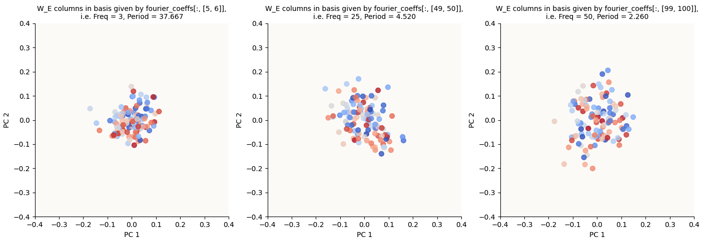 W_E columns in Fourier Coefficient Basis for k in {3, 25, 50} (20,000 epochs)
Notice that they are random and low-magnitude.
5.3. Same Thing (W_L Rows)
The paper mentions that they found the same key frequencies in $W_L$, where:
\[W_L = W_U W_\text{down}\]So, let’s do the same for W_L, which has shape (d_vocab, d_mlp). Let’s first inspect the Fourier Coefficient Norms:
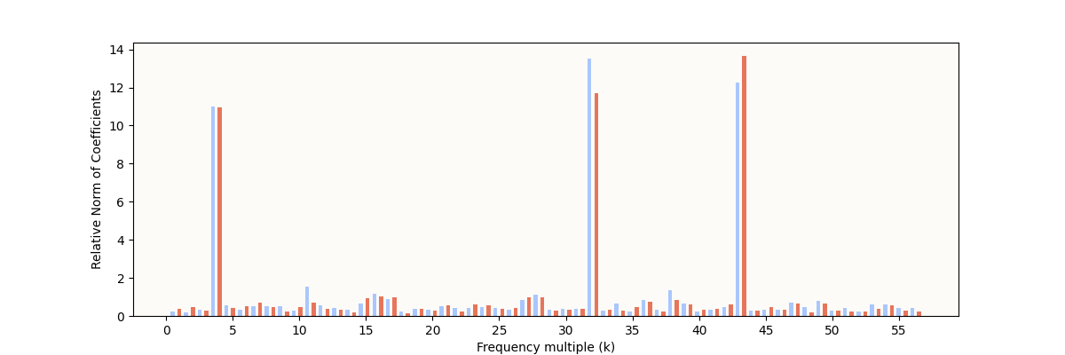 My W_L Fourier Coefficient Norms (20,000 epochs)
And plot our circles:
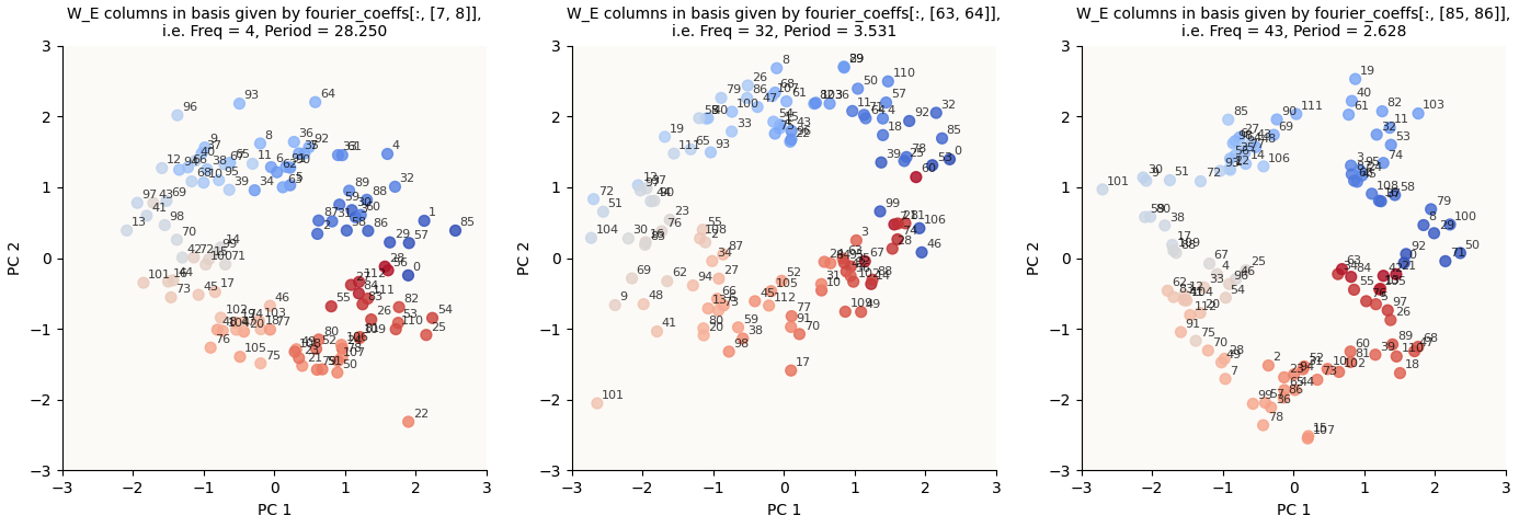 W_L rows in Fourier-Inferred 2D Basis (k Hz Circle), for k in {4, 32, 43} (20,000 epochs)
I should mention that the original paper chose to visualize $W_U W_\text{down}$, even though there is a bias in the MLP down-projection, $b_\text{down}$. The fact that $W_L$ doesn’t take into account $b_\text{down}$ is partially the cause for the extra warped circles here.
6. What Are The Attention Heads Doing?
The next step in figuring out how the model makes use of these circles is to figure out how the circles connect to the MLP block. Let’s take a look at the attention maps for 6 sample pairs for all 4 heads:
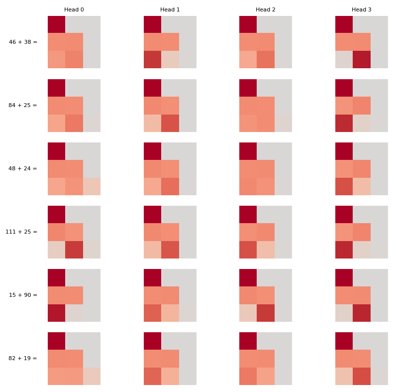 Attention Maps for 6 randomly sampled pairs
Let’s focus on the last row of each map since it tells you where the attention head is focusing on while processing the last token (=). It looks like rubbish. In particular, I was hoping that we’d see that some attention head has learnt to pay equal attention to the first two tokens, and that all other attention heads become useless, but we don’t super see evidence of this.
So where do we go from here? Well, we know that:
- Attention is just something like the relative magnitude of all the $q \cdot k_i$, for some query vector $q$, where $i$ denotes token index.
- $q$ and $k$ are just linear projections of the input vector to the attention blocks (i.e. the vectors in the $\mathbb{R}^{128}$ space where we found circles; henceforth called “embedding space”).
Therefore, if there’s some periodicity in the embedding space, there MUST be some periodicity in the $q$ and $k$ spaces, which means there MUST be some periodicity in the attention maps. Let’s fix one of the numbers (and vary the other) and plot the latest row of the attention maps for a large number of sample pairs:
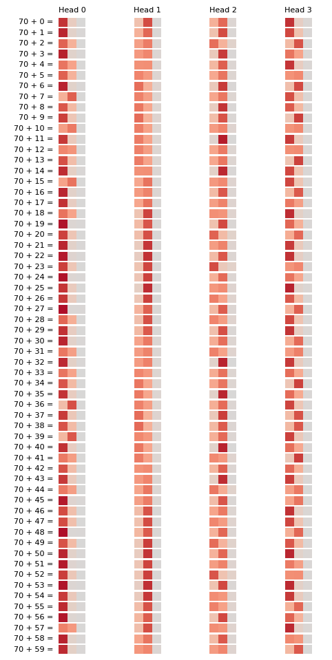 Attention Maps are actually Periodic!
And we see here that the attention maps are indeed periodic! As a bonus, let’s try to do DFT on these to get their primary frequencies.
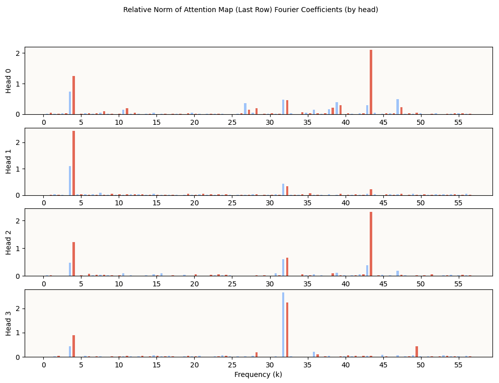 Fourier Coefficient Norms of Attn Activations (Last Row) by Head
You can see that the key frequencies 4, 32, and 43, are distributed over the heads. Some interesting observations include:
- Head 1 is most attuned to the frequency 4, which we can see from the attention maps
- Head 2 and Head 3 are most attuned to the frequencies 43 and 32 respectively, which we can also see from the attention maps
- Head 0 has high-norm coefficients in multiple frequencies, including several non-key frequencies, which interfere to give a non-sinusoidal pattern, which we can also see from the attention maps. It is unclear if the attenuation to multiple frequencies plays some crucial role, or if they’re simply not yet sufficiently decayed.
Crucially, now’s also a good time to point out that the attention patterns are not just periodic when varying b, but also when varying a. This makes sense because a and b are embedded using the same W_E matrix, meaning that they both use the same circle structures in W_E. To see this, we can just visualize the attention score of a (or b, since they approximately sum to 1; I just arbitrarily chose a) in the last row, for all (a, b) pairs:
 Attention Maps are Periodic in ‘a’ and ‘b’
The original Modulo Arithmetic Paper also found such attention maps:
 Original Paper’s Attention Maps are Periodic in ‘a’ and ‘b’ Too
6.1. Periodic Attention on Periodic Embeddings
So we’ve observed that circular / periodic embeddings also mean:
- Periodic $k$, $q$, and $v$ vectors (since each of these are created via linear projections of the embeddings)
- Periodic attention patterns.
So far, we’ve merely replicated and confirmed what the Nanda paper tells us: there are circles in $W_E$, $W_L$, and the attention maps. It’s time to go beyond and see what periodic attention on periodic embeddings means for the attention outputs.
Remember that the attention values ($a_i$, where $i$ denotes token index) all sum to 1, which means that the attention output for token $i$ (call $z_i$), i.e.:
\[\begin{align*} z_i = \sum_{j \leq i} a_j * v_j \end{align*}\]is a convex combination with periodic convex coefficients. In this setting where the attention (when processing the = token) is mostly on the first two tokens (a and b in the equation a + b =), we can roughly simplify this to:
where $x_a$ and $x_b$ are the embeddings for tokens a and b respectively.
For the next step, I wish to see what a periodic convex combination of periodic features looks like. As of yet, we don’t know what $W_V$ is, but we know that it is a simple linear projection, which means it won’t warp the embedding space.
I.E. if a bunch of embeddings formed a circle in the embedding space, applying $W_V$ to them may stretch / squeeze them, but won’t warp them into a non-circle-looking shape like a bean, a knot, a square, or whatnot.
Because a simple linear transformation won’t fundamentally change the shape of the embeddings, and it is the shape that we’re interested in, without loss of generality, I’ll just pretend $W_V$ is the identity matrix. Then, I can just plot $z$ of the = token, given by:
for some periodic $\alpha$. Since Head 1 looks rather much like a simple sinusoidal curve, we’ll just take $\alpha \sim \cos(2 \pi (f + \text{offset}))$ for some frequency $f$. For our plots, we will also fix a (hence $x_a$), and vary b with the same frequency. The actual value for Head 1’s frequency is $4$, but for the sake of illustration, we’ll make it $0.5$.
In fact, depending on how many wavelengths the attention coefficient $\alpha$ is offset (looking at the attention maps above, this offset is itself periodic), we get a whole family of curves!
When the circle (embedding) frequency differs from the attention frequency, we also get different families of curves. For example, if we look at the Fourier-Inferred 2D Subspace (32 Hz) in the attention outputs of Head 1 (which is attuned to the 4 Hz Embedding Circle, hence produces attention scores of 4 Hz), we get different patterns from the above. Below, I illustrate what the attention output ($z$ or $v$; since $z$ vectors are just weighted sums of $v$ vectors, $z$-space and $v$-space are equivalent) should theoretically look like when we visualize the Fourier-Inferred 2D Subspaces (k Hz) of the attention output when the attention head’s frequency ($\alpha$) is different from $k$.
You will see the characteristic petal shapes in all combinations of embedding and attention frequencies. Though not super relevant, I’d point out that when the attention frequency (alpha) is lower than the embedding frequency, you get petals that overlap, whereas when it’s above, you get petals that don’t overlap.
A friend Jacob said they’re reminiscent of trigonometric polar graphs; indeed, the construction of these curves is different but quite similar, and I wonder if there is some profound connection here.
6.2. Petals in Attention Outputs (z; before W_O)?
The above curves are theoretical predictions for what the outputs $z$ (for token =) look like when the attention values are periodic with some frequency (alpha) and the embeddings are periodic with some other frequency (embedding freq), when we fix token a and vary token b. Let’s see if we can actually find these petal shapes in the actual $z$ values for a = 70 (arbitrarily chosen) and b in range(113).
Example: Head 1 on 4 Hz Circle Subspace
In visualizing the attention outputs $z$ (not $o$, i.e. just before applying $W_O$), we have two decisions:
- Which head’s outputs to visualize?
- Which 2D subspace to visualize?
We’ll start with the simplest option of looking at Head 1 (because its attention values are simply periodic in only 4 Hz), and visualize the 2D subspace corresponding to the 4 Hz circle in the embedding space. Now, what does this mean?
Remember that to visualize the 4 Hz circle in the embedding space, we had to use the fourier coefficients to infer a 2D basis:
1
2
3
4
5
6
7
k = 4
fourier_coeffs = W_E @ fourier_basis.T                              # shape (d_model, P)
basis_vecs = fourier_coeffs[:, [1 + 2 * (k - 1), 2 + 2 * (k - 1)]]  # shape (d_model, 2)
basis_vecs_norm = basis_vecs.norm(p=2, dim=0, keepdim=True)
basis_vecs /= basis_vecs_norm                                       # shape (d_model, 2)

circle_coords_to_visualize = W_E.T @ basis_vecs                     # shape (P, 2)
Because the embeddings are transformed via $W_V$ in the attention block, we want to follow these 2 directions through the transformation via $W_V$. The means answering the question: what 2 directions in the $v$ vectors (or $z$ vectors) am I now interested in visualizing (that correspond to basis_vecs prior to applying $W_V$)? Some linear algebra to figure this out:
1
2
3
4
5
6
7
8
9
10
11
12
13
14
15
16
17
18
# This is the computation of v vectors in attn head i
V = W_E @ W_V_head_i                        # eqn shapes: (113, 32) = (113, 128) @ (128, 32)

# We would have wanted to visualize W_E @ basis_vecs.
# Now we only have V, so we have to figure out new_basis to extract from V,
# the equivalent of basis_vecs in W_E
W_E @ basis_vecs = V @ new_basis            # eqn shapes: (113, 128) @ (128, 2) = (113, 32) @ (32, 2)

# Substitute
W_E @ basis_vecs = W_E @ W_V_head_i @ new_basis

# Rearrange
basis_vecs       = W_V_head_i @ new_basis
new_basis        = pseudo_inverse(W_V_head_i) @ basis_vecs
                 = inverse(W_V_head_i.T @ W_V_head_i) @ W_V_head_i.T @ basis_vecs

# Coords to visualize
projected        = z_values @ new_basis     # shape (113, 2)
Above, we predicted that when the embedding circle frequency (4 Hz) is the same as the attention frequency (4 Hz), we’ll get this:
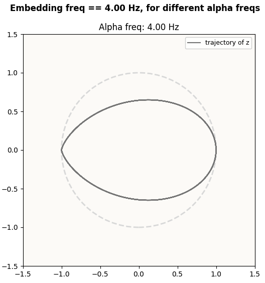 Predicted z pattern in 4 Hz circle space, for 4 Hz attention frequency
Let’s see what actual embeddings we get:
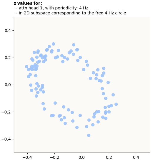 Actual z embeddings in Fourier-Inferred 2D Basis (4 Hz circle), for 4 Hz attention frequency
Example: Head 3 on 4 Hz Circle Subspace
Let’s try another (attention_head, subspace) pair. Let’s try head 3 (attention frequency of 32 Hz) on the 2D subspace corresponding to the 4 Hz embedding circle still,
Prediction:
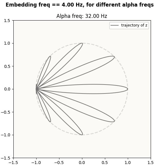 Predicted z pattern in Fourier-Inferred 2D Basis (4 Hz circle), for 32 Hz attention frequency
Actual:
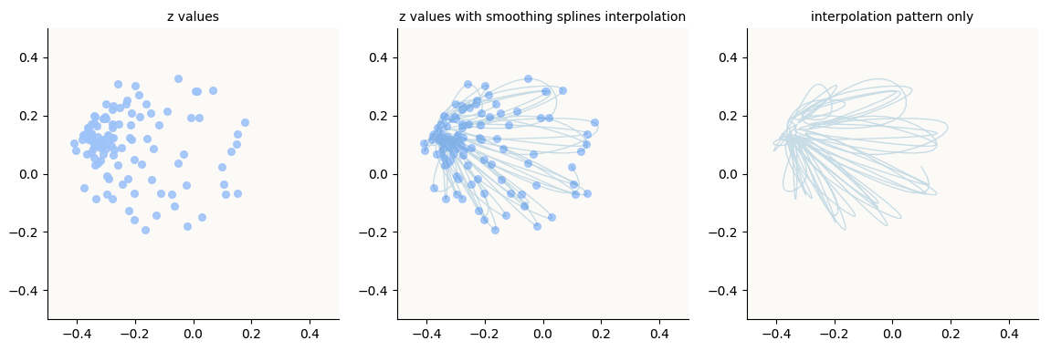 Actual z embeddings in Fourier-Inferred 2D Basis (4 Hz circle), for 32 Hz attention frequency
Example: Head 1 on 32 Hz Circle Subspace
Another one still!
Prediction:
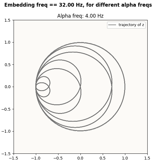 Predicted z pattern in Fourier-Inferred 2D Basis (32 Hz circle), for 4 Hz attention frequency
Actual:
 Actual z embeddings in Fourier-Inferred 2D Basis (32 Hz circle), for 4 Hz attention frequency
I think this is pretty astoundingly beautiful! In particular, nobody has articulated the existence of these multi-lobed petal-like structures in embedding spaces of LLMs even if they’ve discovered the simple circles / periodic structures. These structures are also very surprising to me, because they don’t seem very amenable to linear separation. Representations that sit on the perimeter of a simple circle are not surprising to me because every point can be linearly separated from the rest, and indeed that is what an MLP layer with $\text{ReLU}$ does (refer to “Superposition - An Actual Image of Latent Spaces” for illustrations of this), but the same cannot be said for points that sit on the perimeter of these petal shapes.
7. Petals Interfere to give Simple Circle
By extension, since the attention outputs ($o$) are merely linear projections of $z$ (i.e. $o = W_O \cdot z$), then these petal shapes should remain present in the $o$ space. For good measure, for each attention head individually, I went ahead and did similar visualizations for the head-specific $o$ vectors for all pairs [(70, b) for b in range(113)], and saw the same petal structures.
However, visualizing head by head does not give the full picture of what’s eventually going on in the $o$-space, because you are only considering each individual head’s contribution to the $o$ vectors at any one time. Remember that all the $v$ vectors from each head are stacked, and $W_O$ is applied to that to transform it back to the $\mathbb{R}^{128}$ model space:
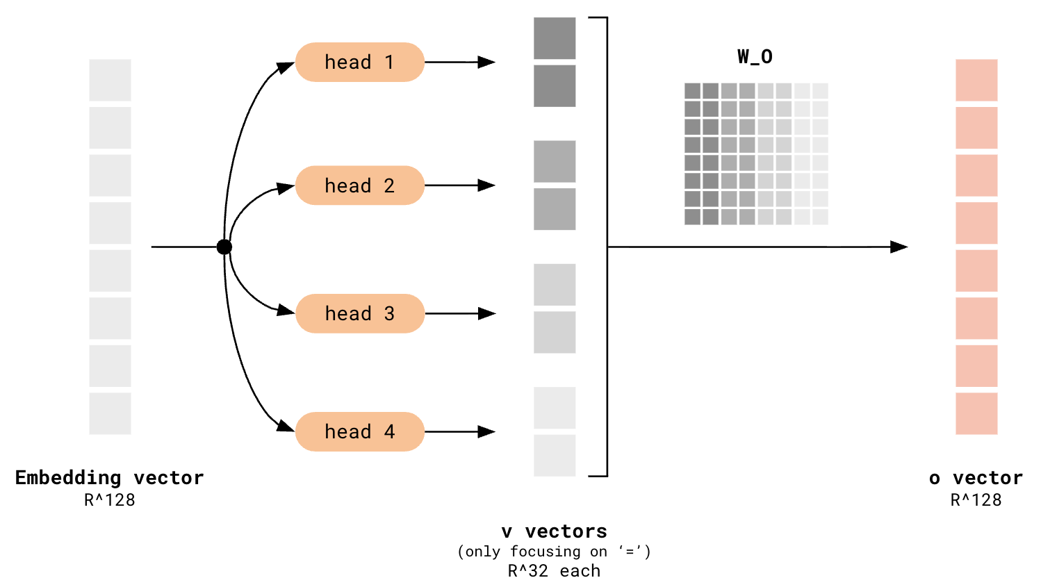 v vectors get stacked, then get transformed by W_O
The application of $W_O$ to the stacked $v$ vectors is equivalent to taking a weighted sum of the columns of $W_O$, where the coefficients are given by the values of the stacked $v$ vectors, so you can see that all the contributions of each attention head are summed together. The consequence of this is that it could well be possible for the contributions from head 2 (e.g.) to disrupt the petal structure contributed by head 1 (e.g.).
7.1. Empirical Evidence
Let’s see how the different heads combine to give a final pattern.
Zoom In: 4 Hz Circle Subspace
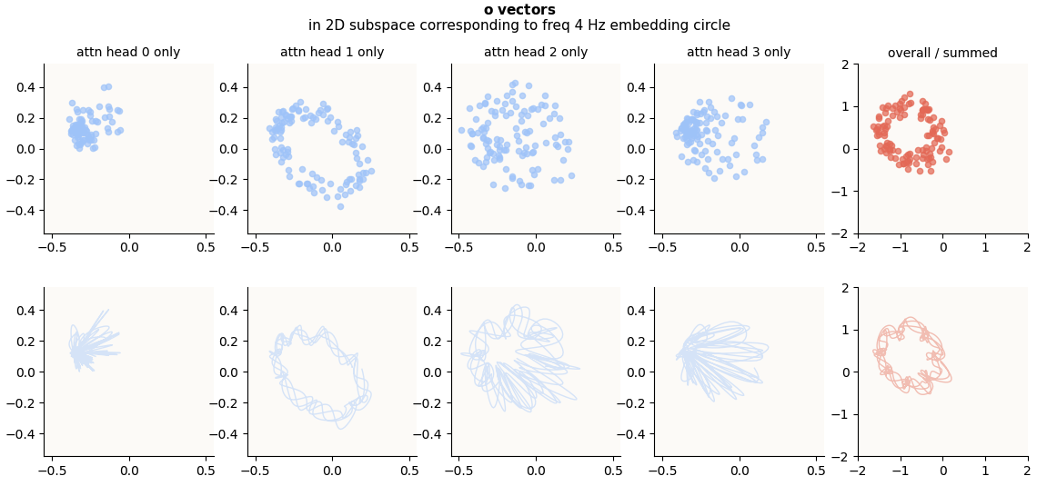
o-vectors corresponding to Fourier-Inferred 2D Subspace (4 Hz Embedding Circle), head-wise and summed
This is quite amazing. The petal structures seems to have disappeared in the aggregate $o$ vectors (red plot), to give a circle! The circle looks very wiggly, and I suspected that it could either be not a circle in actuality, or that it could merely be an artifact of the interpolation being too expressive / overfitting the points, just like in the attn head 1 plot. To be sure, I did a Fourier Decomposition and plotted the norms of the coefficients for each coefficient again for the red points:
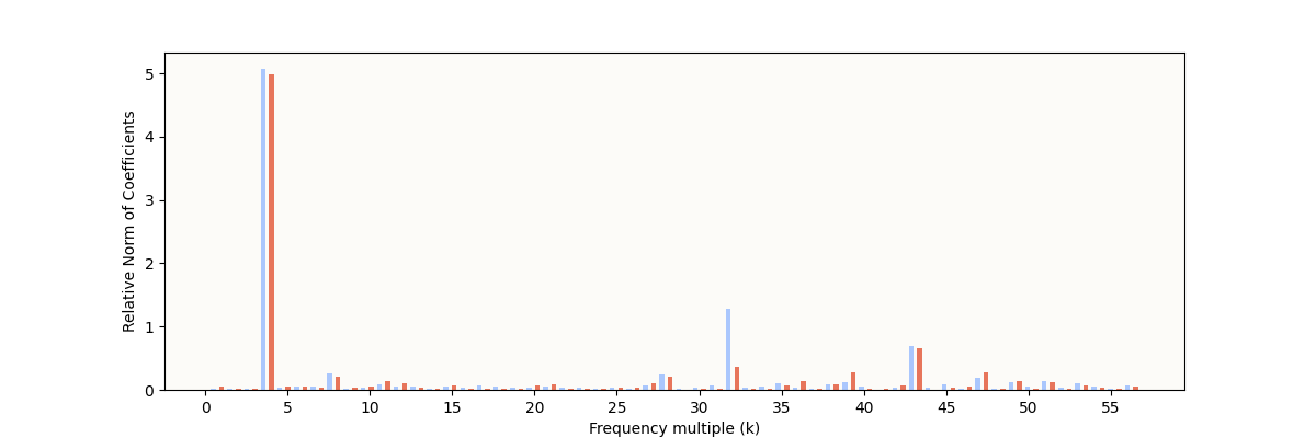 Fourier Coefficient Norms for Projected
 o vectors
With such a dominant 4 Hz component, we are confident that the circle in the red plot is indeed a circle and not some complex petal-shaped curve. So, it’s interesting that these complex petal-shaped curves have recombined to give a circle!
The same thing happens for the 2D subspaces corresponding to the other embedding circles. More visualizations in the next section.
7.2. Petals Shift Over Increasing a to Give Moving Circle
For this next section, I don’t want to just focus on any one given value of a. I want to traverse a sample sequence of a values (each a value still has all b values from [0, 113); that’s how we have 113 points to make up each pattern) and animate how these petal shapes change as a increases, and how they still sum to a circle, and how the circle moves around. The punchline for this section is that the petal shapes always recombine to form a circle, and not that the circle is panning around.
Note: turns out, the panning around of circles is an important thing to understand, but gives an incomplete picture of how the circles vary as a increases. For each of these circles, there exists other subspaces where the petals combine differently to still give a circle, but a circle that rotates, and this rotating circle is the key to modulo arithmetic computation. Because the discovery of this hidden subspace is somewhat involved, I’ll explain this more in Section 9. You will see in Section 9.6 that there is some combination of the patterns in the “panning space” (visualized here) and the hidden rotational space that gives rise to the final rotational circles that are used by $W_U$ to perform the read-out of the correct answer.
4 Hz Circle
Starting with the 4 Hz Circle:
32 Hz Circle Subspace
43 Hz Circle Subspace
Alternative Visualization
Now that we know that these 4 Hz, 32 Hz, and 43 Hz circles exist in the $o$ vectors, we can use another method to try and visualize them. It would simply be what we did at first with W_E and W_L: to run DFT on these $o$ vectors and to project them on the 2 directions given by the 128-dimensional $\sin$ and $\cos$ coefficients corresponding to each of these frequencies. I did them just to make sure that these circles were truly truly present in the $o$ vectors:
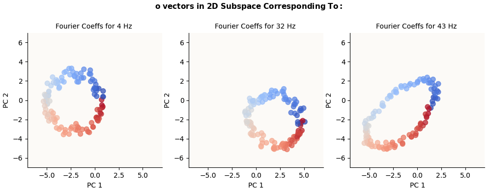
o vectors in Fourier-Inferred 2D Basis (k Hz circle) for k in {4, 32, 43} (alternatively calculated)
I make no comment on why the 43 Hz Circle looks so stretched.
I may have missed a normalization factor somewhere. 🙂
7.3. Why?
To state what we’ve observed so far in simple terms:
- We observed periodic (circular) embeddings
- Periodic embeddings necessarily lead to periodic attention coefficients
- Periodic attention on circular embeddings lead to complex periodic (multi-lobed) value embeddings
- Each attention head has its own multi-lobed structure
- Multi-lobed structures vary based on relationship between embedding circle and attention frequency
- These multi-lobed structures combine to give a simple single-lobed / circular structure in $o$ space again
It would be nice if we could argue that:
- The main goal is to generate simple circles in the $o$ space because they may be particularly amenable to downstream readout functions (MLP layer).
- Embeddings that approximate periodic functions like sines and cosines are especially amenable to composition (constructive interference) to give that desired simple circle, at least if we were only interested in discrete points along the circle. This is essentially the Fourier Decomposition argument again - something like: just like how sines and cosines of different magnitudes and frequencies can combine to give any arbitrary function, multiple instances of the above petal structures (generated the way we generated them) of various orientations and frequency combinations can combine to give any arbitrary function, and particularly, a simple circle.
The above would be a neat argument for why periodic embeddings are learnt, and why there are circles of MULTIPLE frequencies, not just one.
For now, this argumentation remains out of scope of this blog post and we will simply operate from the fact that the petal structures just coalesce to form a simple circle again.
8. How Does MLP Use These Circles?
Gotcha: Do The W_E and o Circles Coexist in the Same Subspace?
Between the attention and MLP blocks, the attention output ($o$) is added to the residual stream, which already contains the original embeddings (columns of W_E), which itself is a circle. The immediate question to ask is: did the newly added $o$ circle interfere with the W_E circle? The only way the 2 circles would meaningfully interact is if they lived in the same subspace. To figure out if any pairs of these basis vectors spanned similar subspaces, for all combination pairs of a set of $o$-derived basis vectors and W_E-derived basis vectors, I plotted the dihedral angle (think of this as the angle between the normals of 2 planes) between them. The dihedral angle is small only if the subspaces are very similar.
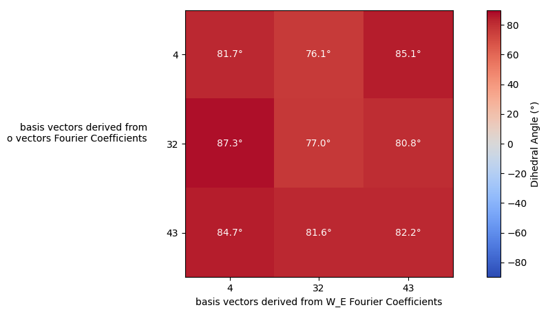 Dihedral Angles of all (W_E basis, o basis) pairs
Ok, none of the pairs have a small dihedral angle, so we know that the $o$ vectors / circles are getting written into a different subspace than the ones that the original W_E circles live in - they don’t interfere.
Guess: W_up Should Have 113 Vectors That Align With o Circles
My initial guess was that I should be able to find a set (or even 3) of 113 vectors that more or less align with the directions of these $o$ vectors that are arranged in a circle. The reasoning behind this is that each one of these W_up vectors should act as a detector for $o$ vectors in that direction and basically produce an activation in one of the 512 elements in the MLP output vector. The MLP output vector will hence have 113 (or 3 sets of 113) positions which each represent 1 number, and W_down can just permute them into the correct position such that the softmax will be able to decode the correct number. However, upon deeper thinking, this wasn’t quite right, for these reasons:
- If this were true, we expect $W_L$ to have a large frequency 1 Hz component, which it doesn’t. Instead, it has the same frequencies as before (4, 32, 43).
- This model actually doesn’t have superposition (!!!)
This Model Doesn’t Have Superposition
The TLDR here is that the MLP block’s $\text{ReLU}$ non-linearity turns out to be non-critical. It could have been spurriously helpful, but a model variant with a $\text{ReLU}$-less MLP turned out to grok modulo arithmetic just fine. This section goes through the discovery of this fact and argumentation of why it makes sense, but feel free to skip.
In “Superposition - An Actual Image of Latent Spaces”, I illustrate how W_up, b_up, and $\text{ReLU}$ can cleverly segment a subspace into 2 regimes (per MLP dimension) in order to silence all other features except the one we care about:
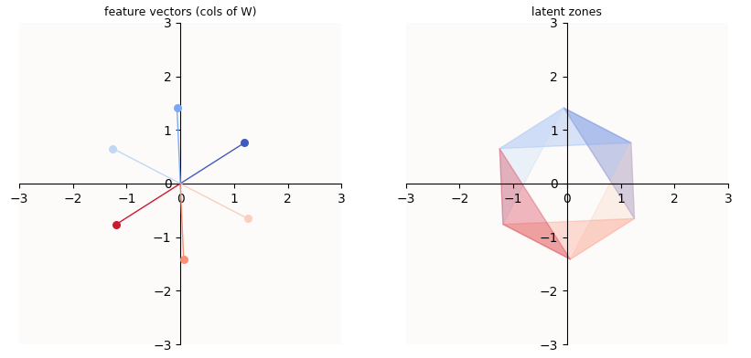 o-vectors corresponding to subspace of 43 Hz Embedding Circle, head-wise and summed
For example, in the above example, unless an embedding were found in the mid-blue region, the post-$\text{ReLU}$ value of that feature will be 0. So, even if you activated the light blue or dark blue feature, unless you STRONGLY activated it, you would still be outside of the mid-blue region, and hence would be zero-ed by $\text{ReLU}$. The orientation of the regions are controlled by W_up and b_up. In particular, the more selective (small) you want region $i$ to be, the more negative b_up[i] has to be.
The above mechanism is how a model is able to store more features (6) than it has dimensions (2). In such a setting, the model is said to exhibit superposition. However, this toy model that we trained here, after the Modulo Arithmetic Paper, does not actually exhibit superposition. Or at least, it doesn’t need to exhibit superposition, because there are only 113 meaningful features the model has to learn (i.e. ['the answer is {c}' for c in range(113)]), which can be contained within the 128 dimensions of the model (d_model).
And so, the MLP block can learn simple linear transformations to maintain the entire geometric structure of the circles WITHOUT making use of $\text{ReLU}$ at all. In such a setting, the model just has to learn positive b_up values in order to shift all the features further into the positive orthant (in the d_mlp = 512-dimensional MLP output space), in order to avoid non-linear distortion by $\textbf{ReLU}$, which happens at the value 0 for all dimensions.
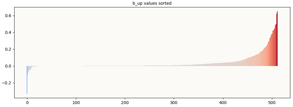
To prove that this is happening, we visualize the b_up values (sorted) and observe that insufficient (way fewer than 113) of them are significantly negative. The negative b_up values are what makes a useful superposition of features possible, and since there are way too few of them, we know that this model is not relying on superposition to encode features.
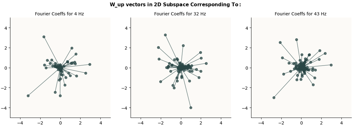
W_up Columns Don’t Line Up With Circle
And indeed, when we plot the 512 columns of W_up in the 2D subspaces that we expect those circles to live (given by the sets of Fourier Coefficients obtained from the $o$ vectors), we don’t see any nice circles:
The MLP Layer Is Just An Affine Transformation
Following the argumentation that d_model = 128 is already sufficient dimensions to encode the 113 features without superposition, the job of the MLP layer isn’t to exploit $\text{ReLU}$ to arrange features in a superposition, but to actually shift the circles into the positive orthant such that they are NOT affected by $\text{ReLU}$. What this entails is adding some offset (which can be done by b_up). Here’s some visual intuition:
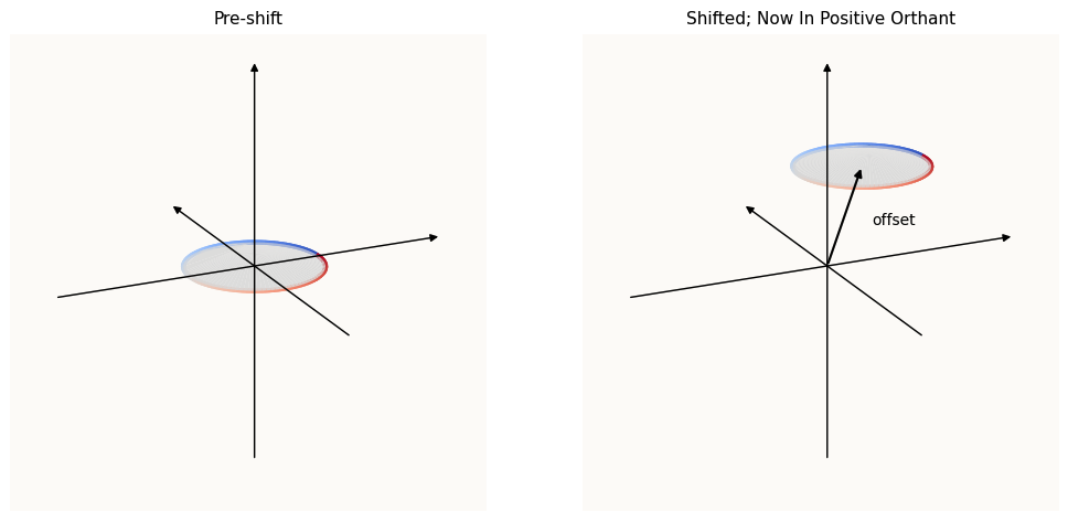 MLP just has to move Circle into Positive Orthant; ReLU not necessary
As proof that the model doesn’t have superposed features / need $\text{ReLU}$, I trained a variant of the toy model without the $\text{ReLU}$ activation function, and it managed to grok Modulo Arithmetic:
 Training Curves of ReLU-less Model Variant
To reiterate, since the MLP block doesn’t actually introduce any meaningful non-linearity to the feature space, we know that the circles are basically preserved through the MLP block. We can see this is true by visualizing the respective 2D circle spaces again (same as before, basis vectors are computed using Fourier Coefficients for these frequencies) and see that the circles are still there:
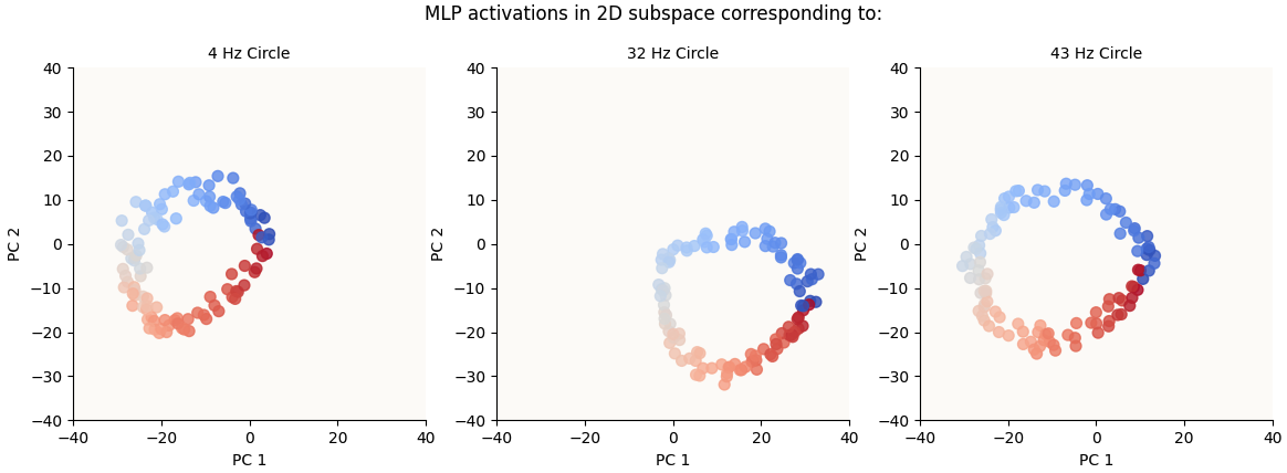 Circles are still there in MLP Activations
9. Rotation of Circles
Now, we know that:
- The number embeddings are periodic, which means that attention values (for any given
a, for all(a, b)pairs) are also periodic - Each attention head outputs different petal structures depending on its attention frequency
- These petal structures sum to form circles again. TLDR: the attention block creates circles via a summation of petals.
- The MLP block is just an affine transformation. This transformation is NOT a function of input data.
- The rows of
W_Lare probes / detectors that infer the answer depending on which numbers in the number circle the rows align most with. The rows ofW_Lare NOT a function of input data.
This means that the computation of the circles output by the attention block are ALL of the meaningful computation of the answer to (a + b) % P = ?. Since this circle has to align with the correct rows of W_L, when we try different values of a and b, we should expect to observe that these circles are rotating in some way.
9.1. o Circles Revolve Around
In Section 7.2, we already discovered that there are circles in the o space, and that they move around. Let’s have another look at the overall circles (without considering the petals) to see how they move. The following animation is similar to before, but here’s how to interpret it anyway:
- 1 frame corresponds to 1 value of
a - Each point in a single frame represents the
ovector of the=token for a particular(a, b)pair. We plot every value ofbfor this value ofa, so each circle is made up of 113 points. - The gradient of each circle represents the increasing values of
b. - The small grey dots are the number embeddings (rows of $W_E$), projected accordingly through $W_V$ and $W_O$.
As you can see, the circles are not rotating. However, they seem to be sliding around the various quadrants / revolving around the origin. Now’s also a good time to remember how these circles were formed - the summation of petal structures (1 per head). The petals are themselves the trajectories traced out by various interpolations between 2 points on the embedding circle (or columns of $W_E$; animation in Section 6.1), which means these individual petal structures are strictly within the confines of the embedding circle. The summation of the petal structures (these circles above) should also hence be within the confines of the embedding circle, magnified by {num_heads} times at most. In this case, you see that the colorful circles are orbiting within the confines of the embedding circle (grey dots).
9.2. o Circles Rotate
Henceforth, any mention of “Singular Vectors” will be interchangeable with “Principal Components”
It turns out that this is a rather misleading way to look at the movement of the circles. Using the Fourier Coefficients to infer a 2D basis for each circle ensures that you will see the circle, but misses out on extra important information. If we were to collect all the pairs of 2D basis vectors (one per value of a), we now have a collection of 2 * len(sample_a_values) vectors, each being d_model-dimensional. If we were to take the Singular Value Decomposition (SVD) of this set of vectors and take the top 2 Singular Vectors / Principal Components (PCs), we would see the circles head-on, much like in the above animations. This is because by construction, the set of d_model-dimensional basis vectors we’ve collected prioritize the visibility of the circles. However, now that we have the entire set of basis vector pairs, the subsequent singular vectors also capture how the circle orientations (i.e. the surface on which the circle lies) change as a changes. It turns out that PCs 3 and 4 (or 2 and 3, 0-indexed) are actually very important too, and I’ll explain the reason later. For now, I simply present these dimensions of the circles:
The key takeaway in this visualization are that:
- The orbit isn’t as pronounced. One may conclude that either there’s no orbit, or if there is, instead of orbiting a center that is outside the circle, the center is now inside the circle.
- There is rotation (!!!)
9.3. Rotation + Revolution
For this next part, I’ll plot the circles in the MLP activation (post-$\text{ReLU}$) space, instead of the o space. The affine transformations in the MLP block do some stretching / reflection of the o space, which makes the visualizations clearer, but for the most part, the dimensions are still partitioned pretty nicely into the “Revolution Space” (first 2 Singular Vector Directions / Principal Components) and the “Rotation Space” (second 2 Principal Components). To satisfy our curiosity, let’s just see what this looks like, as best as we can (in 3D), for a chosen circle (4 Hz circle).
9.4. Discovering The Relevance of Fourth PC
This section is about how I discovered that the third (and fourth) Principal Components were important. Feel free to skip.
If we were to stick with only the 2D visualization of the MLP Activation circles, we’d see that the circles seem to move (revolve) around a center point that was outside the circles, without any rotation. However, the MLP output circles (after applying W_down and b_down) seem to have no revolution (they’re always in the center), but they now have a rotation. I didn’t understand how a simple affine transformation could achieve that, so I tried to examine W_down to see if I could construct a simplified version of it and see what it was doing.
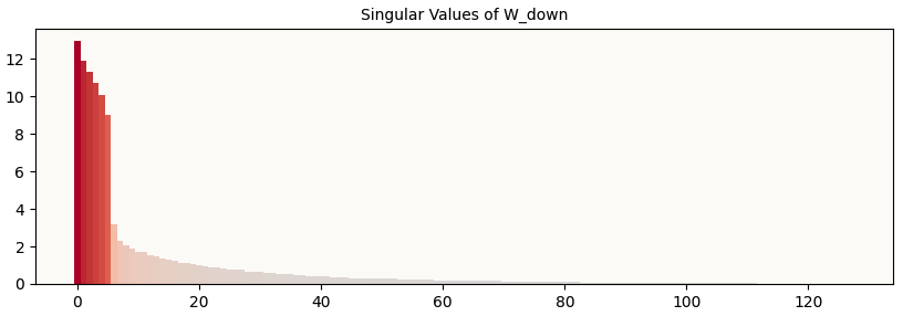
I first took a look at the singular values of W_down:
And noticed that there were only 6 of them that were large. This roughly maps onto the fact that we have 3 sets of circles, each living in a different 2D subspace. I then did guess-and-check to see if I could map on pairs of singular vectors onto the 3 sets of circles. I arrived at a pretty good guess:
And I tried to see what these 2 singular vectors of W_down corresponded to in terms of the singular vectors of the MLP activations, so I plotted the cosine similarity between each pair of W_down rows (i.e. singular vectors [3, 5], [1, 2], [0, 4]) and the first 6 (arbitrarily chosen) singular vectors of the MLP activations:
 The relevant
 W_down Rows are Similar to 3rd and 4th top Singular Vectors of MLP_activations
And here I can see that it largely ignored the plane of orbit (first 2 PCs of MLP activations) and focused instead on the vertical axis (3rd PC of MLP activations) and the mysterious 4th singular vector of MLP activations.
So, what if we just visualized the MLP activations in their 3rd and 4th PCs?
We get the purely rotational (as opposed to revolutionary) circles. And this is how we know that the rotational components are the 3rd and 4th PCs.
9.5. Summary: MLP Just Focuses On Rotational Component
The TLDR from “Section 9.4” is that the MLP block magnifies and focuses on the 3rd and 4th PCs of each set of Fourier-Inferred 2D bases (1 set per k-Hz circle). These (‘magnifies’, ‘focuses’, ‘PCs’, ‘Fourier-Inferred 2D bases’) are all a chain of linear / affine operations, and the last animation of Section 9.4 pretty much shows the rotating ring that is fed into the final transformation matrix: W_U, up to some minor translation and perturbations.
To be sure, let’s look at the circles that W_U gets to see (i.e. the MLP_output vectors):
9.6. What Created The Rotational Component?
We saw that the rotation circles were present in the MLP activation vectors, and also the $o$ vectors. This means that the attention block, which generates the $o$ vectors, created the rotating circles. However, previously in Section 7.2, we visualized a 2D subspace that showed us a revolving (and not rotating) circle. What’s left is just to see how the rotating circles got created by the attention block.
Well, we know that the rotating circles lived in a somewhat unexpected 2D subspace of the MLP activation vectors (the 3rd and 4th PCs of all the Fourier-Inferred 2D Subspaces combined). Then, we traced the 3rd and 4th PCs in the MLP activation space back to the $o$ space, visualized those dimensions, and saw the rotating circles. We can further trace this hidden subspace back to each head’s $z$ space and visualize those and see how they combine to give the overall rotating circles in the $o$ space.
Let’s interpret this:
- You can still see the characteristic petal shapes per head. This is expected we’re merely adopting another point of view, compared to Section 7.2
- The orientation of the petals are no longer the same across heads. To observe this, let’s focus on the 4 Hz circle. We see that in attention heads 0, 2, and 3, the start of the petal structure (red points meeting the blue points) are facing the right, whereas in attention head 1, the start of the petal structure is facing up. This is in contrast to Section 7.2, where the petal structures in all heads had the same orientation.
I’ll reiterate that the first 4 columns literally sum (simple sum) to give the last column. Without getting too into the weeds, it is obvious that the combination of different orientations and scales of these petal structures allow for these various petal structures to sum to a rotating circle.
We’ve observed first hand how these strictly panning, non-rotational components can sum to a rotational circle. We hence can also assume that the panning components visualized in Section 7.2 contribute to this summation to make the eventual rotating circles we visualized in the MLP activation vectors (Section 9.4, Section 9.5), which are much more regular and circular.
Indeed, if we were to ablate (project out) the first 4 principle components from the attention outputs using this matrix:
\[\begin{align*} M_\text{ablate} = (I - X(X^\top X)^{-1}X^\top) \end{align*}\]where the columns of $X$ contained the top 4 PCs collected from the set of Fourier-Inferred 2D basis (either from MLP activations or pre-ReLU vectors) for each circle frequency (hence a total of 12 vectors), we see the test accuracy drop from 100% to 0.91%, or a score of 116 / 12769, which is chance.
So there we have it. The meat of the entire computation (i.e. formation of circles that can rotate), other than the embedding and read-out function, was basically done in the attention block.
10. Read-Out Transformation: W_U
By now it should be pretty obvious that W_U (I’ll call this “decoder”) simply has to align itself with the circles found in the MLP output space.
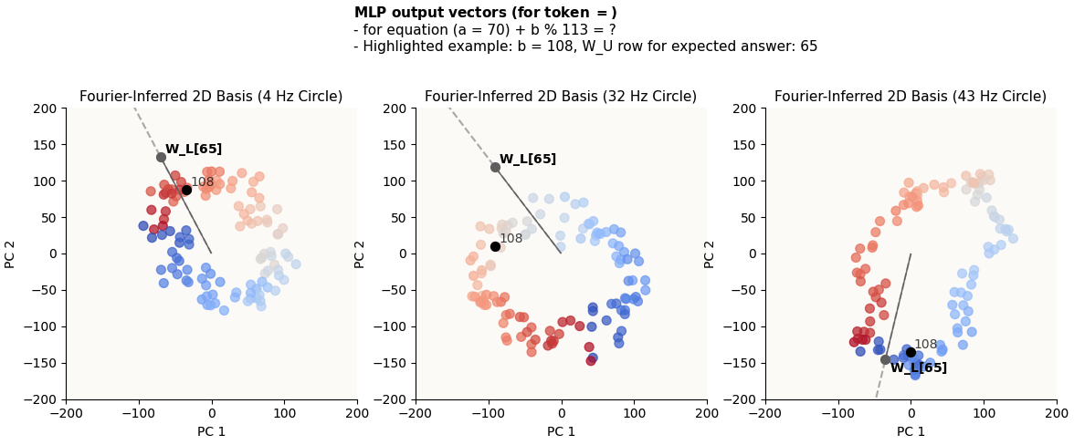
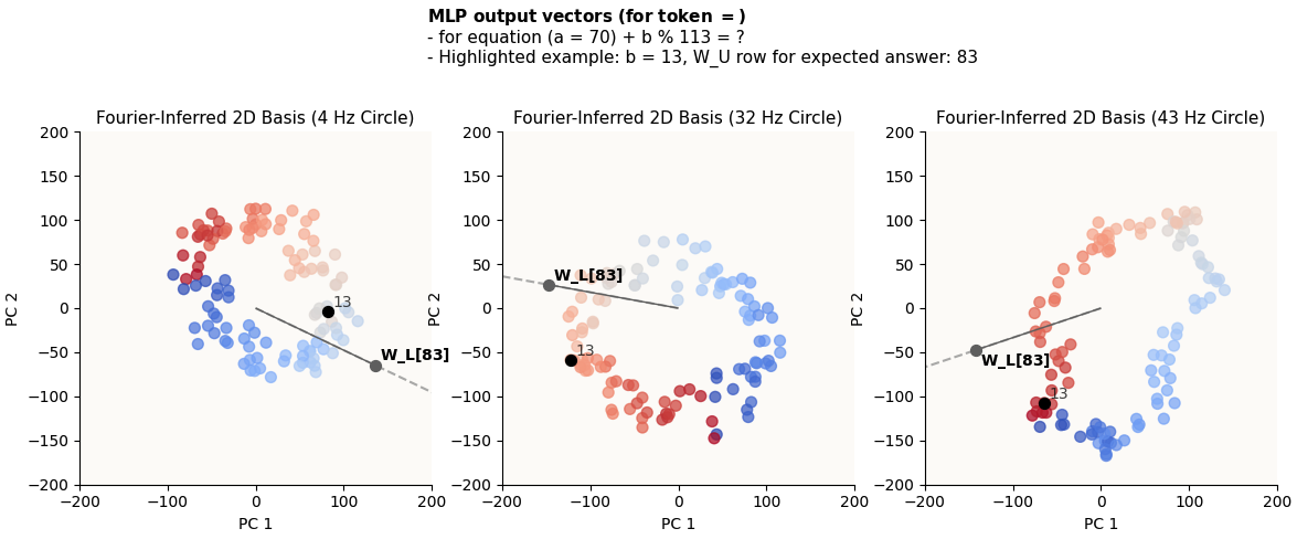
What do I mean by this? Let’s look at some examples of how the row of W_U corresponding to the expected answer lines up with the MLP output vectors for the = tokens for some a and b pairs:
70 + 108 = 65
70 + 13 = 83
Remember that each colored dot represents a different value of b. You can see that for any chosen b value, that dot will be relatively highly in the direction of W_L[{expected_answer}] (call this “highly activating of the correct answer”). It doesn’t matter that it’s not the dot that’s the MOST in the direction of W_L[{expected_answer}], because it is unlikely that its competitors will also be highly activating of the correct answer in the other circles, because the circles are of unsynchronized frequencies, and ultimately the cumulative effects of alignment across all circles will still favor the correct answer.
11. Implications on Circle Multiplicities and Frequencies
11.1. How Many Circles?
How many circles must the model learn, and what kinds of frequencies must the circles have?
Theoretically, the model could learn just 1 circle, and have the frequency be 1 Hz. However, this circle would have to be PERFECT, i.e. all the embeddings sit nicely on the perimeter of the circle, such that every point is linearly separable from the rest. This way, you can define rows of W_L that can cleanly align with the correct embeddings, meaning that the MLP_out embedding for = for a certain (a, b) pair will be the most highly activating embedding of the correct row of W_L.
However, having just 1 circle is not possible. This is due to the fact that these circles have to rotate / revolve, and such rotation / revolution is only possible due to the circles being a summation of multiple petal structures, and to have multiple petal structures, you must have $>= 2$ attention heads, with each attention head having different attention frequencies, which necessitates $>= 2$ embedding circles, each with different frequencies.
11.2. Relationship of Circle Frequencies
Remember that circles (given that they are circles) can be defined by either their sine or cosine component. These circle frequencies must be such that the summed sine (or cosine) wave functions have frequency 1 (one circle is completed over P tokens). The requirement is that $P \times \text{GreatestCommonDivisor}(k_1, k_2, \cdots,) = 1$. The easiest way to achieve this is to just have the frequencies (or periods) be co-prime, and can be done with just 2 circles.


