Multi-Layer Latent Space Visualization

In MLPs, What Input Gives What Output?

If you had a series of MLP (nn.Linear) layers chained together, you may like to answer the question: if I wanted the final layer outputs’ first element (call $h_1$) to be activated (i.e. $> 0$), what would my input have to be?

To set the stage, one may ask: who cares? Well, wouldn’t it be great if you could answer: I want a model’s response to my one-word prompt to be a certain word (e.g. “extermination”), what should my one-word prompt be? Or perhaps, I want my text-to-image model to produce an image that is a little more {insert description of feature 16243, or whatever}, what can I say to make it do that? To do so requires us to know how to pass constraints on the output (i.e. desired properties of the output) all the way back to the input space. Modern models are not just MLP blocks - there are blocks like Attention, Convolution, Diffusion, that all complicate matters, but they do all have MLP blocks. This makes this reverse engineering process in pure-MLP toy models worth studying.

But is that even calculable? How would we do that? Generally, only bijective (one-to-one) functions are reversible, and many models do contain many-to-one components, namely the $\text{ReLU}$ activation function, causing many to think that reverse engineering inputs from desired outputs is not possible. Indeed, most of deep models (linear transformations) is reversible, which leaves the main challenge to be $\text{ReLU}$. While reverse-engineering the exact inputs from a desired output is not possible, reverse-engineering a range of input values is very possible. In fact, the way that $\text{ReLU}$ is usually used (following an up-projection from d_small to d_large), makes it such that the degrees of freedom in the range of possible inputs is only d_small, which is much smaller than d_large. This makes the range of input values that could give a desired value in the output space much more constrained and useful. However, doing so turns out to be rather computationally expensive. This blog post introduces and walks through the logic of computing an “un-$\text{ReLU}$” operation, and talks about how one may implement this exponentially expensive operation.

Example Of Reverse-Engineered Inputs

Linear transformations interspersed with non-linearities are what make up the backbone of all deep models. If you wanted to reverse-engineer inputs based on some desired output, you can’t really escape this simplification model of deep models. Hence, we’ll think of this simplified model of multi-layered MLPs:

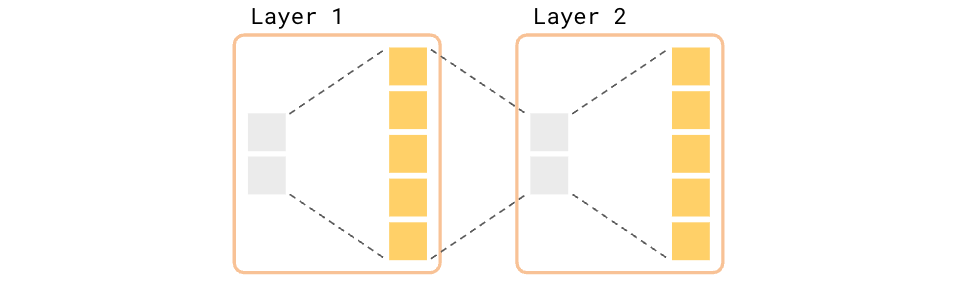2 Layer MLP (Simplified)

I.E. each layer is doing an up-projection (d_small --> d_large), followed by $\text{ReLU}$, followed by a down-projection (d_large --> d_small). For the last layer, we don’t do a down-projection, as it is usually the post-$\text{ReLU}$ “features” (or “neurons”) that we care about.

If we have d_small = 2 and d_large = 10, a question we might want to answer is: where must we be in the input 2D space in order to have the first element of the 10D input be $> 0$? Our goal is to be able to describe the region such as this:

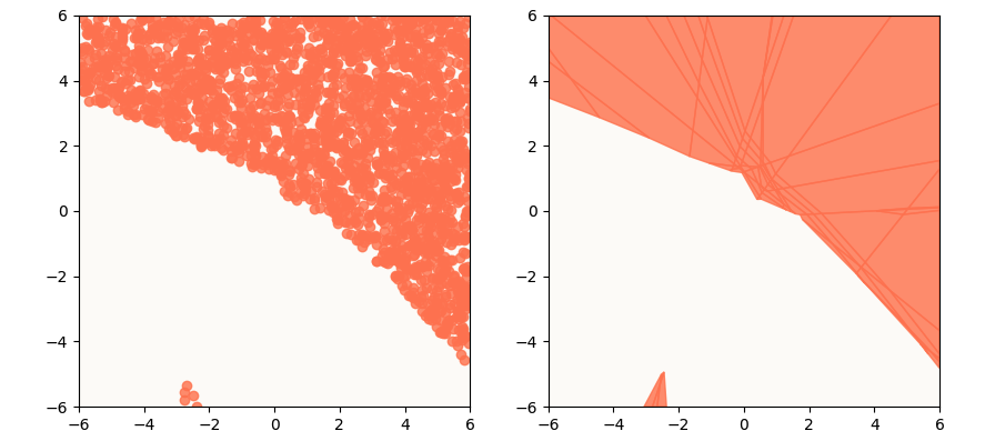Regions in 2D Input Space that will Activate First Element of Output

To generate the left plot, I uniformly sampled points between [-6, -6] and [6, 6] and plotted only those that gave a positive output[0]. The right plot is an analytically computed “activation zone” wherein inputs will produce outputs with positive first values. Each one of these “tiles” is described using a conjunction of linear inequalities.

You may ask: well, it seems like we get a pretty good idea of where in the input space our inputs have to be in order to generate a desired output property just by uniformly sampling a bunch of input points and surveying their corresponding outputs (i.e. do what I did for the left plot above), why is that insufficient? It’s because this provides a very incomplete understanding of the input space. In particular, there can be a large number of disjoint activation zones, and they can be anywhere in the input space. It is likely (and exponentially likely as dimensionality grows) that your sampled inputs are not diverse enough to discover all activation zones.

For example, if we had just sampled from [-4, -4] to [4, 4] in this case, we wouldn’t have discovered that small island at the bottom. If we wanted to figure out activation zones for the sake of knowing whether or not it is possible at all for a model to exhibit a certain behavior, we need a complete list of activation zones. Expressing each tile / activation zone as a conjunction of linear inequalities also makes it convenient for us to return a sample point within the tile, using standard Linear Programming (LP) methods.

Visualizing a Latent Space

Deep models are all performing some sort of information compression. A useful way to think about the latent space of models (usually refers to the residual stream of Large Language Models, or the grey 2-vectors in the graphics above) is as a “superposition of features,” for which there is much research material. In “Superposition - An Actual Image of Latent Spaces”, I introduce a method to visualize such features. The method relies on the fact that $\text{ReLU}$ effectively segments a lower-dimension (2D in this case) subspace into a superposition of 5 half-space pairs (5 because the up-projection projects the 2D subspace to a 5D subspace in this case).

Here’s what would happen if we chose one latent space (2D) to visualize, with respect to features determined by an immediate up-projection + $\text{ReLU}$:

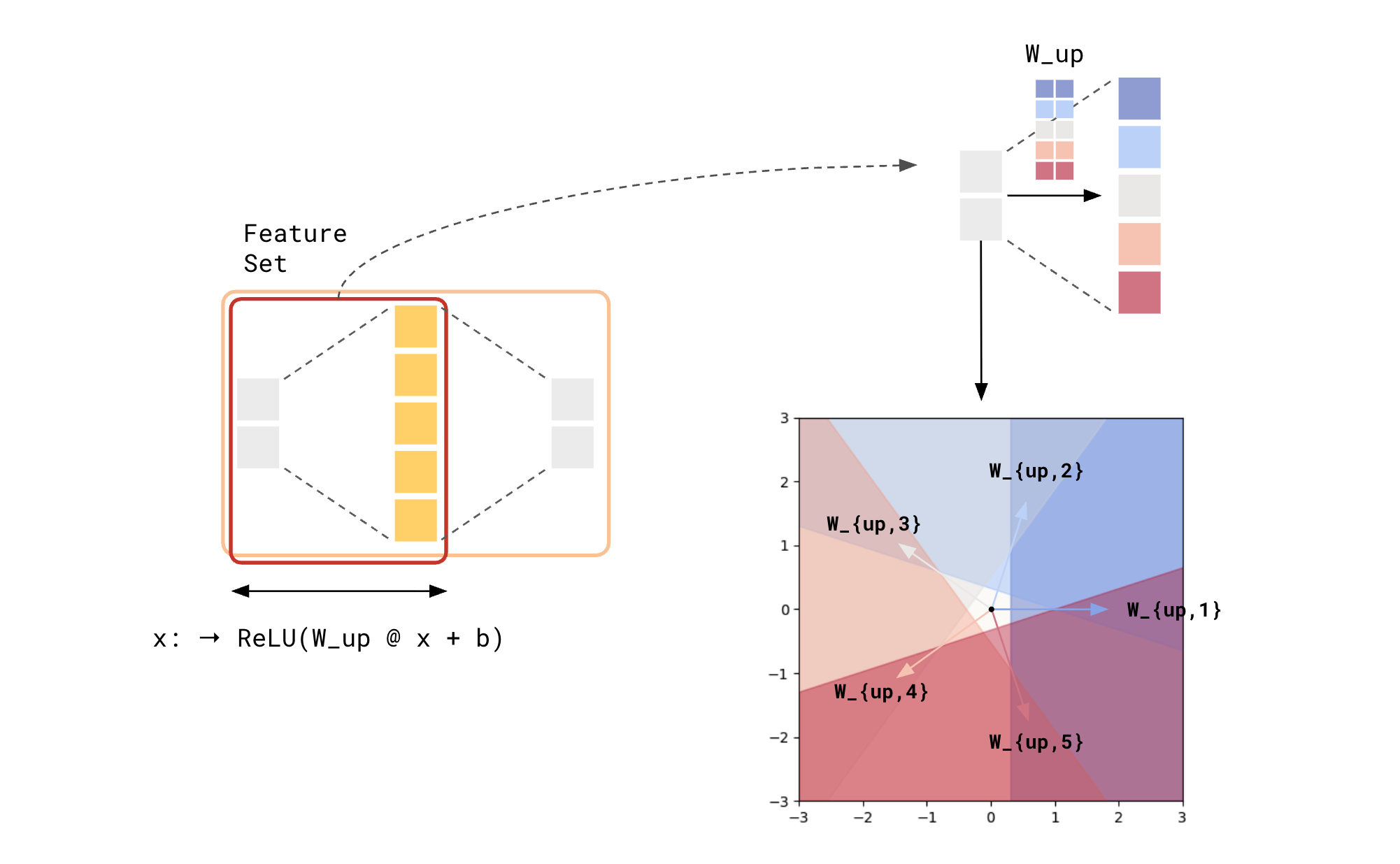Latent Space Visualization for 1-layer MLP

Note: the regions are determined by the rows of W_up (color-coded vector arrows) as well as b. For more information on how this is done, read “Superposition - An Actual Image of Latent Spaces”

Latent Spaces for Chained MLPs

The above plot gives you an idea of where you have to be in the 2D space in order to activate any subset of the 5 features. Now, let’s attempt to ask the same question for chained MLPs - given 2 consecutive MLP layers, where would you have to be in the earlier 2D space to activate any subset of the 5 features of the later MLP block?

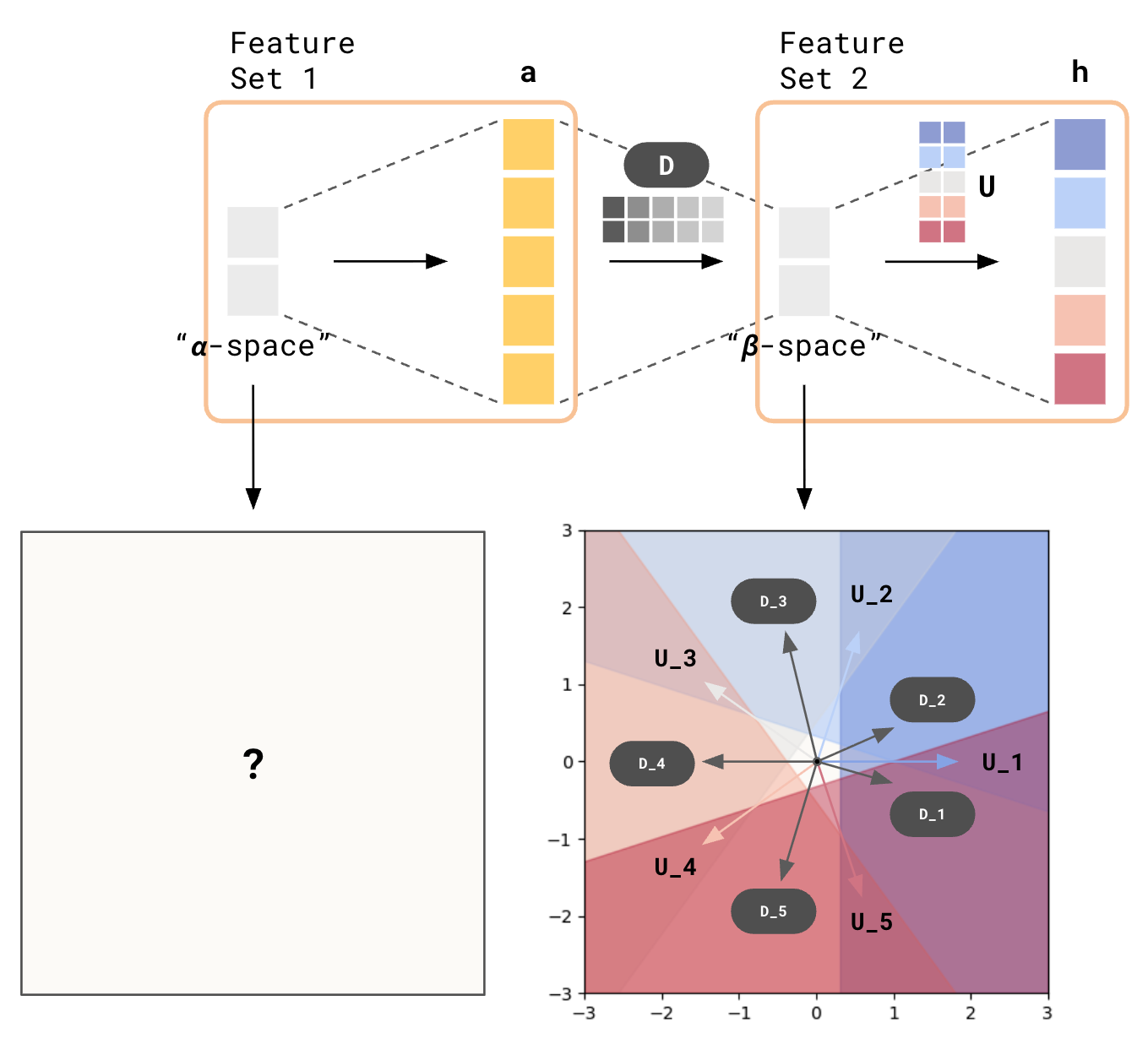Latent Space Visualization for 2 chained MLPs?

For example, for our final output to activate the 1st feature (i.e. $h_1 > 0$), it must be in the blue zone (pointed to by $U_1$) of the 2D input space of Feature Set 2, which I’ll call “$\beta$-space.”

In turn, what would it take to be embedded onto the blue zone of $\beta$-space? Where in $\alpha$-space must I be for that to happen?

Problem Setup

To figure out how to do this, we will walk through an example with d_small = 2 and d_large = 3, so that we can visualize things. This will give us an impression that things are simpler than they are, so I’ll take extra care to reason out what things should be when the dimensionalities are much larger than we can visualize.

Terminology:

Layer 1

\[\begin{align*} a &= \text{ReLU}(W x + b_W) \\ z &= Da \\ \text{where } x & \in \mathbb{R}^2, a \in \mathbb{R}^3, z \in \mathbb{R}^2 \end{align*}\]

Layer 2

\[\begin{align*} h &= \text{ReLU}(U z + b_U) \\ \text{where } h & \in \mathbb{R}^3 \end{align*}\]

Known Sample Weights W, D, U

For the sake of simplicity and clarity of visualization, let’s choose $W$, $D$, $U$ to be regular shapes (triangles), and biases to be the dense negative vector of arbitrary magnitudes.

\[\begin{align*} U = \begin{bmatrix} 1 & 0 \\ -\frac{1}{2} & \frac{\sqrt{3}}{2} \\ \frac{1}{2} & -\frac{\sqrt{3}}{2} \end{bmatrix}, & \text{ } b_U = \begin{bmatrix} -0.3 \\ -0.3 \\ -0.3 \end{bmatrix}, \\ D = \begin{bmatrix} \frac{1}{2} & \frac{1}{2} & -\frac{\sqrt{3}}{2} \\ \frac{\sqrt{3}}{2} & - \frac{\sqrt{3}}{2} & 0 \end{bmatrix}, & \text{ } b_D = \begin{bmatrix} 0.0 \\ 0.0 \\ \end{bmatrix}, \\ W = U, & \text{ } b_W = \begin{bmatrix} -0.5 \\ -0.5 \\ \end{bmatrix}, \\ \end{align*}\]

Reverse Engineering Layer 2

Let’s begin reverse engineering. The goal is to activate the first feature of $h$, i.e. $h_1 > 0$. Since we have to start from the last layer (layer 2), let’s visualize what $\beta$-space looks like, together with the rows of $U$ drawn:

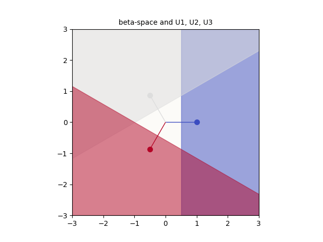Beta-space with U1, U2, U3

How do we interpret this? If we wanted to activate $h_1$, the embedding ($a$) would have to be in the blue zone. This makes sense, because $h_1$ $= \text{ReLU}($$U_1$ $a \text{ } + $ $b_{U,1}$$)$, which means that $a$’s dot product with $U_1$ must be greater than $-b_{U,1}$.

How did we get this? In “Superposition - An Actual Image of Latent Spaces”, I describe at a high level how $\text{ReLU}$ produces latent zones like these, but I didn’t formally describe the reversal of $\text{ReLU}$ in full detail. I will do it now.

Starting Constraint:

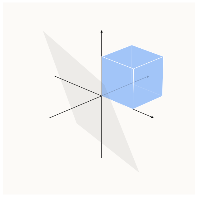
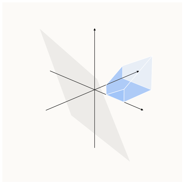
\[h_1 > 0\]

If we were to visualize what this looks like within a cubic volume of space centered at the origin, this is it:

Initial Constraint: h_1 > 0

This is basically saying, post-$\text{ReLU}$, we need our points in the above blue zone.

Reverse Up-Proj + ReLU

However, notice that not all points in the blue zone are possible, because $\text{ReLU}$ constraints values to be $\geq 0$. So, we need to take the intersection of the above constraint, and the $\text{ReLU}$ constraints, which is simply that $I z \geq 0$, or the positive orthant:

Intersection of h_1 > 0 and Positive Orthant Constraints, which is just Positive Orthant Constraints (subset)

Then, notice that the equation involving $\text{ReLU}$ is this:

\[\begin{align*} h &= \text{ReLU}\left(U z + b_U\right) \end{align*}\]

This means that the domain that $\text{ReLU}$ is operating on isn’t the entirety of $\mathbb{R}^3$, but just the span of the columns of $U$ (i.e. the Range of $U$). If we were to plot this plane out together with the above constrained area, we get:

Let’s visualize un-$\text{ReLU}$-ing 1 dimension of this positive orthant at a time. This corresponds to focusing on the face of the positive orthant where only that dimension is 0, and projecting it along the negative direction in that dimension back onto the Range of $U$.

We can’t un-$\text{ReLU}$ dimension 0 because we require $h_1 > 0$ (strict inequality).

Similarly, let’s visualize un-$\text{ReLU}$-ing 2 dimensions of this positive orthant at a time. This corresponds to focusing on in the axial lines of the positive orthant where 2 out of the 3 dimensions are 0, and projecting it along the negative direction in both the zeroed-out dimensions, onto the Range of $U$.

We can’t un-$\text{ReLU}$ dimension sets (0, 1) and (0, 2) because they both require dimension 0 to be $0$, which is against $h_1 > 0$.

Also, not shown here, is the un-$\text{ReLU}$ of the full dimension set (all 3 dimensions at once; which involves un-projecting the origin vertex of the positive hypercube, which is inadmissible because we require $h_1 > 0$), as well as the the empty dimension set (nothing to un-$\text{ReLU}$; trivial).

In this case, we find that all our pieces nicely form a union that just describes a simple half-space:

3 Pieces Form 1 Half-space

Mathematically, we will treat this as a single half-space, as it is convenient to work with only 1 linear inequality as opposed to 3 sets (for this example). However, the fact that these pieces come together so nicely is not guaranteed, and in writing a procedure to perform un-$\text{ReLU}$, you’ll have to treat them as 3 separate pieces. This single inequality is simply:

\[\begin{align*} (Da) \cdot U_1 + b_{U, 1} > 0 \end{align*}\]

And this is our starting point for reverse-engineering Layer 1.

Reverse Engineering Layer 1

Remember, we chose $D$ (arbitrarily) to be:

\[\begin{align*} D = 0.5 \times \begin{bmatrix} \frac{1}{2} & \frac{1}{2} & -\frac{\sqrt{3}}{2} \\ \frac{\sqrt{3}}{2} & - \frac{\sqrt{3}}{2} & 0 \end{bmatrix} \end{align*}\]

And we know the values of $U$ and $b_U$.

Reverse Down-Proj

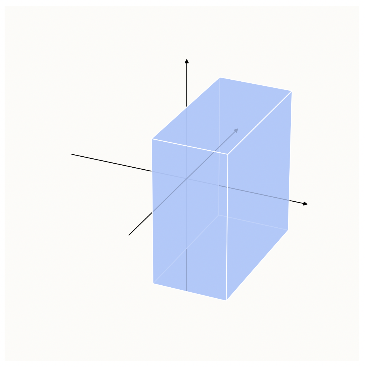
Re-arranging the above constraint to be more explicitly in terms of $a$ instead of $(Da)$, we get:

\[\begin{align*} \text{} \\ (U_1^\top D) a + b_\text{U, 1} & > 0 \\ \Longrightarrow \left( \begin{bmatrix} \frac{1}{4} & \frac{1}{4} & -\frac{\sqrt{3}}{4} \\ \end{bmatrix} \right) a - 0.3 & > 0 \end{align*}\]

This corresponds to a half-space in 3D. The below image illustrates what imposing this half-space constraint onto a cubic volume of space looks like:

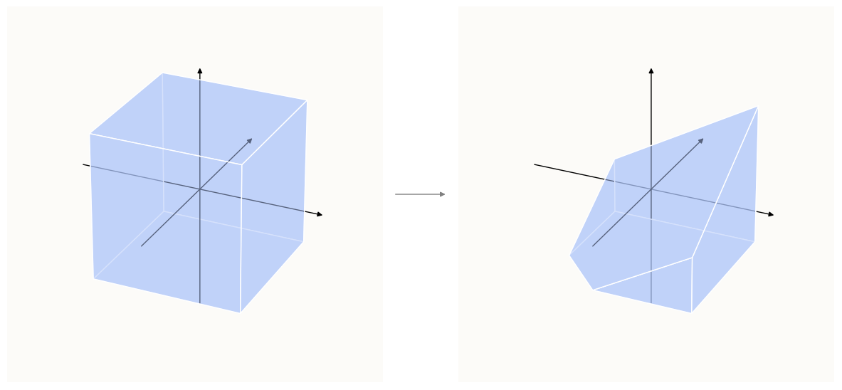Origin-centered cube gets cut by Constraint Due To h1

Reverse Up-Proj + ReLU

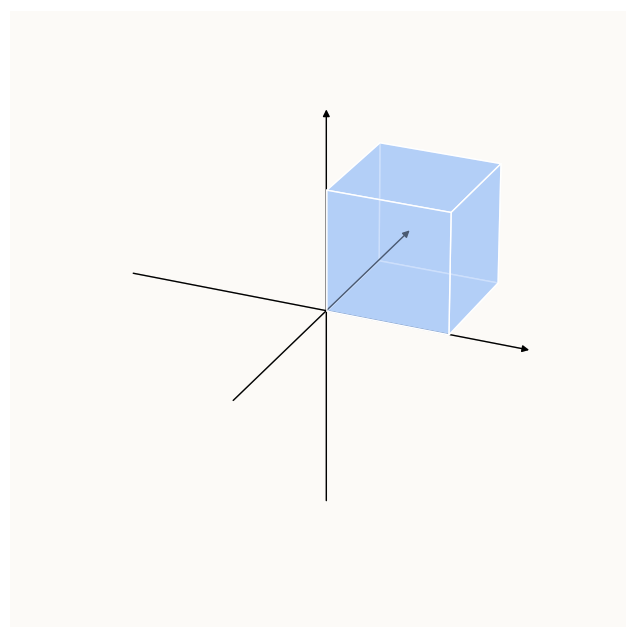
Remember that we also have the Constraints Due To $\text{ReLU}$, which essentially limits us to the positive orthant (hypercube):

Origin-centered cube is limited to positive orthant after imposing Constraint Due To ReLU

Combining (taking the intersection of) all the above half-spaces induced by their constraints, we get:

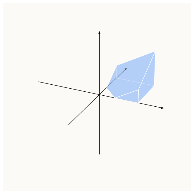a has to live somewhere in this space

Similar to before, let’s plot the plane given by $W$ (a.k.a. Range of $W$) in and realize that we only have these axial surfaces (and edges) to consider:

Only the darker surfaces (axial planes) are accessible

If we were to propagate it back to before the $\text{ReLU}$, sort of undoing the projection onto the surfaces of the positive orthant that $\text{ReLU}$ does, we end up with the following, which I’ve broken down into 2 phases for clarity. The first phase involves un-$\text{ReLU}$-ing 1 dimension at a time so that the relationship between the pre and post-$\text{ReLU}$ regions is geometrically clear, and the second phase involves doing the rest.

Above shows “phase 1,” where we Un-$\text{ReLU}$ the faces (only 1 dimension had been zero-ed by $\text{ReLU}$). This is more intuitive.

Above shows “phase 2,” where we Un-$\text{ReLU}$ everything else (multiple dimensions had been zero-ed by $\text{ReLU}$). This is less obvious because there are multiple projections going on.

Let’s fact check. If we had a model as such:

\[\begin{align*} f(x) & = \text{ReLU} \left( U \cdot D \cdot \text{ReLU} \left( W x + b_W \right) + b_U \right) \text{, with:} \\ W & = \begin{bmatrix} 1 & 0 \\ - \frac{1}{2} & \frac{\sqrt{3}}{2} \\ - \frac{1}{2} & - \frac{\sqrt{3}}{3} \end{bmatrix}, b_W = \begin{bmatrix} -0.5 \\ -0.5 \\ -0.5 \end{bmatrix} \text{, } \\ D & = \begin{bmatrix} \frac{1}{4} & \frac{\sqrt{3}}{4} \\ \frac{1}{4} & -\frac{\sqrt{3}}{2} \\ - \frac{\sqrt{3}}{4} & 0 \end{bmatrix}, \\ U & = \begin{bmatrix} 1 & 0 \\ - \frac{1}{2} & \frac{\sqrt{3}}{2} \\ - \frac{1}{2} & - \frac{\sqrt{3}}{3} \end{bmatrix}, b_U = \begin{bmatrix} -0.3 \\ -0.3 \\ -0.3 \end{bmatrix} \text{, } \\ \end{align*}\]

(all the parameters are as illustrated above), then if we were to randomly sample a whole bunch of 2-D points uniformly from $[-5, -5]$ to $[5, 5]$, i.e.

num_samples = 10000
dim = 2
X = torch.rand(num_samples, dim) * (2 * 5) - 5

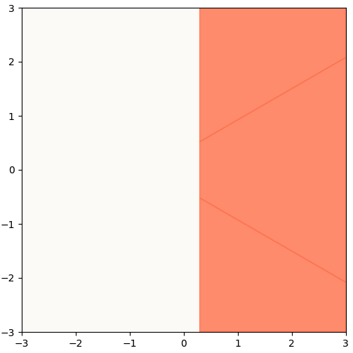
and send those points through the network $f$, and plot only those points that had a non-zero activation for feature 1 (i.e. $h_1 > 0$), we get:

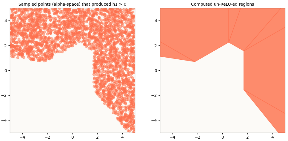(Left) Only sample points that produced h1 > 0. (Right) Our un-ReLU-ed regions.

Does This Scale?

Because we’d like to be able to do this algorithm for any number of layers, let’s write out the necessary ingredients at each step of the way to figure out what our latent activation zones look like. This will also allow us to determine what the computational complexity is. We will compute what it takes to find the latent activation zone corresponding to just one end feature (in this case, it was $h_1$).

Mapping out $\beta$-space

• Latent activation zone was a simple half-space defined by just 1 linear inequality ($U_1 \cdot x + b_{U, 1} > 0$)

Mapping out $\alpha$-space, after having done $\beta$-space

• First, we have to propagate $\beta$-space back to $a$-space (not $\alpha$-space)! This corresponds to the truncated cube as shown above, which is made by the above constraint (linearly transformed by $W$), and the 3 $\text{ReLU}$ constraints. This is dim + 1 contraints.
• Then, we have to figure out how to map this to $\alpha$-space. This is difficult. When you think about what $\text{ReLU}$ does to a dim-dimensional vector, there are basically 2 ** dim different regimes you have to think about. For example, the regime where (pre-$\text{ReLU}$) dim[0] < 0 and dim[1:] >= 0 (only the first element is negative) is different from the regime where dim[-1] < 0 and dim[:-1] >= 0 (only the last element is negative). Of these regimes, only 2 regimes are ignorable: the one where all elements are negative (trivial), and the one where all elements are positive (un-encodable after $\text{ReLU}$). So, you have (2 ** dim) - 2 regimes, within which there could be an activation zone that is defined by up to dim + 1 constraints. This is $O(2^\text{dim})$ computational complexity.

This corresponds to the above example, where we expect (2 ** 3) - 2 = 6 regions, but we only had 5, because the regime corresponding to $x \geq 0, z \geq 0$ did not have an activation zone.

Mapping out to pre-$\alpha$-space: $\gamma$-space

Now with $O(2^\text{dim})$ activation zones in $\alpha$-space, you can imagine that if we were to do the same steps to back-propagate these activation zones back by 1 more MLP block (to a “pre-$\alpha$-space,” which I’ll just call $\gamma$-space). Each of the $O(2^\text{dim})$ activation zones would form a new set of constraints with $\text{ReLU}$, which would result in potentially another $O(2^\text{dim})$ latent activation zones in $\gamma$-space. You can see how this becomes $O(2^{2 \times \text{dim}})$ latent activation zones. The number of zones you’d have to track is essentially $O(2^{L \times \text{dim}})$, where $L$ is the number of layers.

Unavoidably Exponential

You may wonder: why are tracking all these latent activation zones separately even though are (or at least seem to be) contiguous? Couldn’t we combine some of them, or better yet, just record their vertices, and do away with the potentially exponential number of zones? The problem here is that every step of the back-propagation across spaces requires us to do projections to compute points of intersection. These points of intersection are easiest obtained by solving the system of linear inqualities that describe the region, and if you have a non-convex region, you can’t have a consistent set of linear inequalities that describe the entire region. They must be thought of as the union of convex sub-regions.

Also, if you think about what $\text{ReLU}$ does, it splits every dimension of a latent space into 2 regimes, one silent one (for the negative values of the domain), and one linear one. If you have dim dimensions, then naturally you can have up to 2 ** dim different regimes, which is why even simple non-linearities like $\text{ReLU}$ are so powerful. You will never be able to side-step the problem of having $O(2^\text{dim})$ regions of space to reason about.

Intractible

Having walked through the technique one would use to back-propagate constraints on the output space all the way back to the output space, we observe how the number of constraints end up exploding, especially after just a small number of layers for a production model with many dimensions. I initially shelved this, but some friends at Tessel AI wanted to put this to the test on their feature extractors, so I ended up building it. Feel free to contact me if you’d like to find out more.

Call for Optimizations

I spent a LOT of time thinking about what optimizations can be made, especially in the step where we basically iterate over all the orthants to compute the un-$\text{ReLU}$ projection (this section). A lot of my thinking went in the direction of pruning the search space, because not all orthants contain pre-$\text{ReLU}$ images of the polytope that is in the positive orthant. In fact, very few do. However, I couldn’t find any way to reliably prune half or more of the search space. This factor of half is very important, because anything less than that is unsufficient to offset the base-2 exponential complexity of this algorithm. Perhaps some day I’d come back to this and write up all my attempts in full detail, but until then, I would love to hear your thoughts.