In my previous post, “Superposition - An Actual Image of Latent Spaces”, I illustrate how the parameters of a toy ReLU auto-encoder ($W$, $b$, and $\text{ReLU}$), work together to allow models represent more features than they have latent dimensions and reconstruct said features with no loss. That post ends with an actual plot illustrating the latent zones of such a model, which offers a visualization of what ReLU model latent spaces look like, and crystal clear geometric intuition for why they look the way they do.

That sets us up for the real investigative work I’ve been wanting to do: Optimization Failure.

Introduction

In one of their smaller papers - “Superposition, Memorization, and Double Descent”, Anthropic investigated how model features were learnt over time under different dataset size regimes. They trained a toy ReLU autoencoder (a model that compresses an input vector from higher dimensionality to a lower dimensional latent space via weight matrix $W$, and then tries to reconstruct it by applying $W^\top$, adding a bias $b$, and finally, $\text{ReLU}$-ing it). It is a very very interesting paper, but what really caught my attention is a side question that concerns the geometric arrangement of features.

This post will focus on the representation of features / examples. In particular, we see the beautiful geometric arrangement of examples, where each example is assigned a direction, and the directions are as spaced out as possible in the latent space:

In this post, I will treat “examples” and “features” as interchangeable, because I will be using a toy dataset where there will be exactly 1 example of each feature; in that sense, examples are just instances of features.

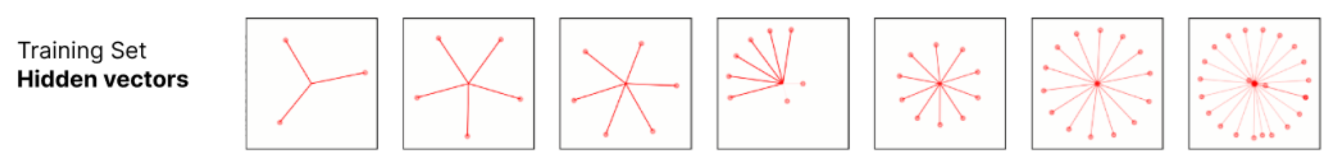Each vector corresponds to a training example in latent space, over a range of dataset sizes (Anthropic)

Intuitively, this all makes sense - the model wants to represent what it learns with as little interference as possible, so it tries to space everything out as much as possible in its latent space, but appealing to this intuition is way too anthropomorphic and doesn’t give us a good enough picture of why there’s this regular geometric arrangement, and when / how this regular geometry is broken.

In particular, there are is a spin-off work / question that was mentioned at the end of the Anthropic post, which caught my eye:

Screenshot of an interesting follow-up work cited by Anthropic

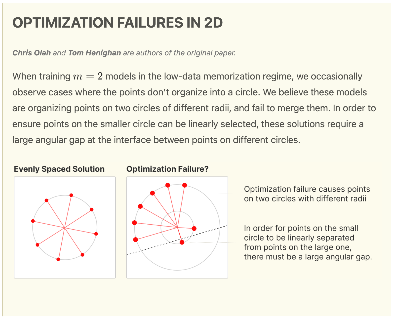
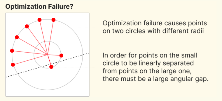
This post is also mentioned as the “Two Circle” Phenomenon in Anthropic’s Circuits Updates - May 2023. There are 3 claims here that I think are faulty:

The models are organizing points on two circles of different radii. I question both the claims of “two” and “circles”, explicitly because it does not seem like two is a special number, nor that features are in general arranged as circles, despite how reminiscent of electron / nuclear energy levels this is.
The models “fail” to merge the multiple circles - it seems to me that if the model indeed differentiated features into multiple “energy levels” such as these, it is not so much that the model wants to merge the multiple circles, but that the multiple “circles” is a desirable property.
“To ensure points on the smaller circle can be linearly selected, these solutions require a large angular gap at the interface between points on different circles”. In general, this seems plausible, but offers very little specificity on what constitutes a large enough phase angle, how linearly separable is considered linearly separable enough, and so on.

TLDR, I find this spinoff question particularly interesting because there are obvious unknowns. Not to shade the researchers (I consider them to be some of the best, field-defining interpretability researchers), but because they only offer intuitive explanations without any justification, for such behavior that could have many intuitively plausible explanations, these claims are particularly feature. In any case, uncovering the mechanical forces behind the geometric arrangement of features and what causes the nice geometry to break in “Optimization Failure” will be illuminating in understanding why models represent features the way they do.

The Questions

Based on their very short write-up above, these questions seem natural to investigate:

Why do points organize themselves into a circle in the ideal case? By circle, I mean with equal magnitude and equally spaced apart.
When do points not organize themselves into a circle?
What are key features of the “Optimization Failure” solution? Is it having multiple circles of different radii? How linearly separable must each point be from the rest of the points?

This post will turn into a bit of a rabbit-hole deep-dive, but I hope to put in my most lucid insights that I have managed to hallucinate over the past months, that I believe will be crucial in attaining a good intuition of how models represent features.

The Problem Set-Up

Anthropic’s Problem Set-Up

I’ll do a very quick summary of Anthropic’s Toy Model set up, and only for the variant I’m interested in. As mentioned, they define a toy ReLU autoencoder that tries to reconstruct $x$, call the reconstruction $y$, by doing the following:

\[y = \text{ReLU}(W^\top W x + b)\]

Where $x \in \mathbb{R}^n, W \in \mathbb{R}^{m \times n}$. $n$ refers to the data’s dimensionality (input dimensionality) and is much higher than $m$, which is the latent dimensionality (aka “hidden dimensionality”).

There is also a sparsity level of $S = 0.999$, which means that every entry of each data sample has a $0.999$ chance of being $0$, and being uniformly sampled from $(0, 1]$ otherwise. After sampling, these data vectors are normalized to have magnitude 1.

Lastly, they define their dataset to have $T$ examples, which is varied from very small ($3$) to very large (million, or infinity, since they generate new data on the fly).

Our Problem Set-Up

We stick to the same toy model, but focus on the case of $n > 2, m = 2$. We will not have a sparsity parameter, but simply have all data samples be perfectly sparse (1-hot) vectors. This is because, while Anthropic was investigating the effect of sparsity on whether or not the model would eventually learn to superpose features or drop features that it had no capacity to express, I want to simply focus on the case where we know that a solution that perfectly superposes all features is possible. This is exactly the case where all input features are perfectly sparse (each data sample has only 1 feature active); this is corroborated by the fact that Anthropic found superposition starts to occur at low enough values of $S$ where the mode number of features active in any given input $x$ is 1.

Moreover, because I don’t want the model to prefer learning any feature(s) over others, instead of having a variable ($T$) number of samples, I give it the same number of examples per feature. My dataset $X$ is hence the identity matrix, where there’s just 1 example per feature (1-hot) vector.

Does the Optimization Failure solution pursue linear separability?

This is probably the easiest question to answer, and is basically answered the moment we have geometric intuition for what the latent space looks like (highly recommend reading my last post for building this geometric intuition). I’m particularly interested in this question because Olah and Henighan claim that in the case of Optimization Failure, “in order for points on the small circle to be linearly separated from points on the large one, there must be a large angular gap.”

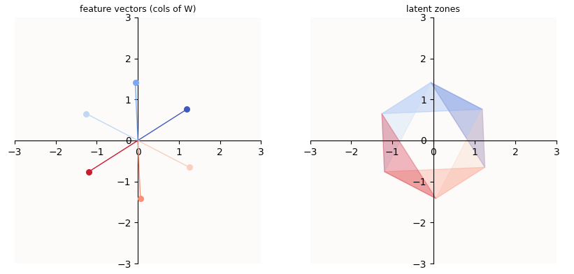
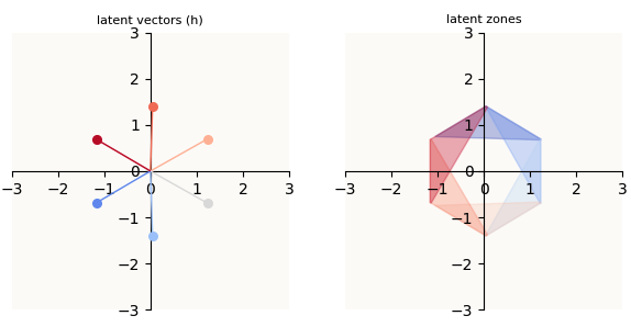
To briefly summarize “Superposition - An Actual Image of Latent Spaces”, the latent space of such an auto-encoder (and $m=2$-dimensional object (plane) living in $n$-dimensional space), looks like this:

In the above example, I trained a bunch of $n=6, m=2$ autoencoders, and selected one where the model learnt to perfectly reconstruct all features. On the left, you can see the column vectors of $W$ arranged into a perfect circle. On the right, I plotted the regions of the latent space (2-dimensional) that correspond to an activation of the $i$-th feature. For example, in order to activate (reconstruct) the orange feature in the reconstructed vector, the hidden vector computed by the model needs to be in the orange region.

Plotting quirks: Notice that the latent space seems to be limited to a hexagon, rather than the entire 2D subspace. This is merely a quirk of my plotting logic; since the non-zero entries of our input vectors (the standard basis vectors) are all $1$’s, it is sufficient to plot a portion of the latent space that contains all the columns of $W$ in 2D (equivalent: all the columns of $WI$ in $n$-dimensional latent space). Such a portion of space is simply given by the outline drawn by enumerating the columns of $W$ in a clockwise fashion.

Occasionally, you will also see that there is a kink in the shape, so instead of expecting a nice hexagon (or heptagon) for 7 points, you may observe an “indented pac-man”. This is simply because there is a point that is so near to the origin (the mouth of the pac-man) that connecting all the 7 points results in a pac-man shape.

To fully appreciate why the activation zones are as such, I illustrate the latent space (a planar hexagon) in a 3D space:

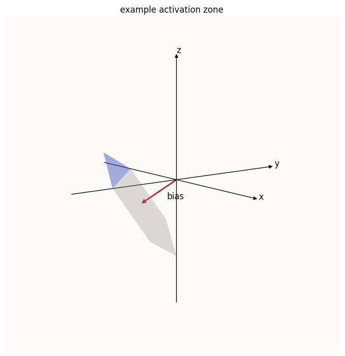
I’ve also highlighted the activation zone of the $z$-th feature, which is simply the part of the latent space with $z > 0$. It is now also obvious that the $z$-th value of the bias is the lever which controls where that blue sliver starts. A $b_z$ that is more negative means that the latent hexagon is pushed down further along the $z$-axis, meaning that the sliver of the hexagon that satisfies $z > 0$ starts further up the hexagon. Conversely, a less negative $b_z$ means that the hexagon will be situated further up the $z$-axis, meaning that the sliver of the hexagon that satisfies $z > 0$ will start nearer the bottom of the hexagon.

I’d also like to point out that the amount of reconstruction a feature gets is hence determined by how much the feature vector extends into its corresponding latent zone:

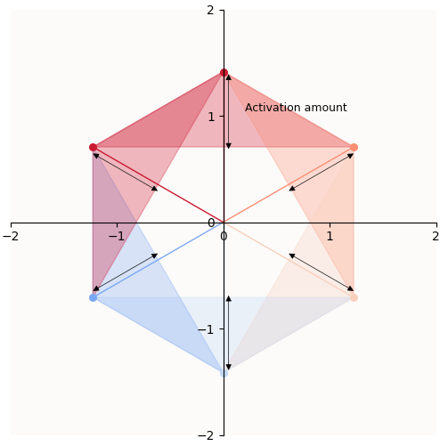Amount of activation must be equivalent to reconstruction of the feature

What this means is that the width of the activation zone (annotated by “Activation amount” in the above plot) directly depends on the amount of feature contruction you want to have. Explicitly, because our vectors are 1-hot, this is our requirement:

\[\text{Reconstruction of feature i when it's active } = W_i^\top W_i + b_i = 1\]

When you plot the columns of $W_i$ onto a 2D plot like we did above, it is also deceptive because this latent space is angled in a specific manner with respect to all the $n = 6$ axial lines, so some feature vectors are more parallel / perpendicular to some axial lines than others, and have a greater / lower component in that dimension than others. For example, if the plane were completely perpendicular to dim $1$, then no matter how long feature vector $W_1$ is, it would never have any component lying in the dim $1$ direction. Conversely, if the plane were completely parallel to dim $1$, then all of $W_1$ would be in the dim $1$ direction. Hence, there is also a scaling factor along each of the 6 directions for the relationship between the magnitude of $W_i$ and the activation amount in the $i$-th direction, and that scaling factor is $\in [0, 1]$.

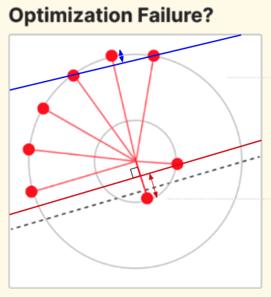
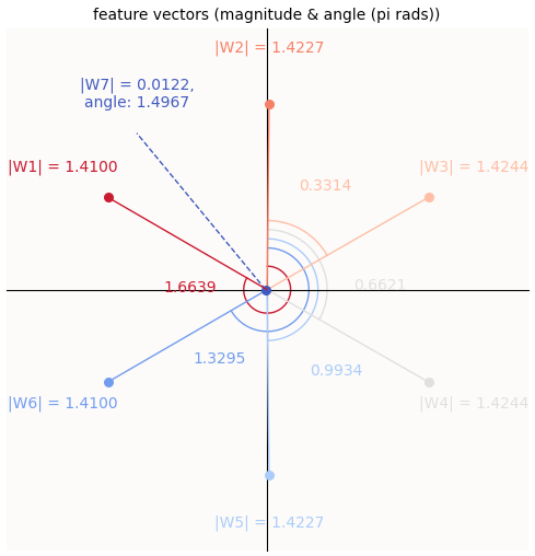
So, in response to whether or not optimization pursues linear separability, the answer is yes, but there’s a lot more nuance to it than is let on by Olah’s and Henighan’s illustration, which I paste below again:

The dotted line linearly separates the one short feature from the rest, yes, but in a rather abitrary way, and doesn’t illustrate how much linear separation is enough, and the point at which linear separation starts to count. Applying our intuition of latent zones and activation amount, we can draw in the real line of separation, which is also where the latent zones start. I’ve drawn one for a short feature and one for a long feature:

You may notice that the activation amount for the long feature seems much less than the activation amount for the short feature - doesn’t this mean that the reconstructed value for the long feature is less than the reconstructed value of the short feature? E.g., if distance annotated by the red double-ended arrow correspond to a reconstructed value of $1$, wouldn’t the distanced annotated by the blue arrow correspond to a value of much less than $1$?
Nope, because of the hidden scaling factors w.r.t to each of these 8 dimensions, mentioned above! Keep in mind that the reconstructed value of feature $i$ is merely the extent to which feature vector $i$ is in the latent zone, in the $i$-th dimension. In a perfectly symmetric latent set-up, the latent plane is tilted equally in all dimensions, but in this asymmetric set-up, the latent plane is tilted much more in the dimensions of the long features (i.e. much more parallel to the long features). You will get a more complete picture of “tilt” in the coming sections.

Why do Features Organize Themselves into a Circle?

TLDR: they don’t have to! Now that we know what our toy ReLU model’s latent space looks like, and that attaining sufficient reconstruction for each feature is really the only goal of the model, we can see that there are many equally good solutions that the model can learn. The most visually and mathematically pleasing one is of course when all features are more or less the same length, and they are equally spaced apart, where all of the $b_i$ values are the same, giving them equal amounts of reconstruction. But, the “Optimization Failure” case of having asymmetric feature vectors is equally “good,” by the measure reconstruction loss. It’s just that because the shorter features mean that the latent space has less of a component in their respective dimensions, the width of their latent zones need to be larger, such that they can still have the same amount of reconstruction in those dimensions.

Optimization Failure Mode: Symmetric Failure

So, if a model can achieve a symmetric configuration, why does it sometimes fall into the asymmetric “Optimization Failure” mode? To find out, we first look at when a model fails completely to learn a feature (call this “Symmetric Failure”). There are only a few ways optimization can fail for this toy model. In Olah’s and Henighan’s screenshot, the model is obviously asymmetrical and turns out, lots of model latents become asymmetrical in Optimization Failure, but it seems to me that all “failed” models have at some point passed through the “Symmetric Failure” mode before turning asymmetrical. Let’s take a look at what this “Symmetric Failure” mode looks like.

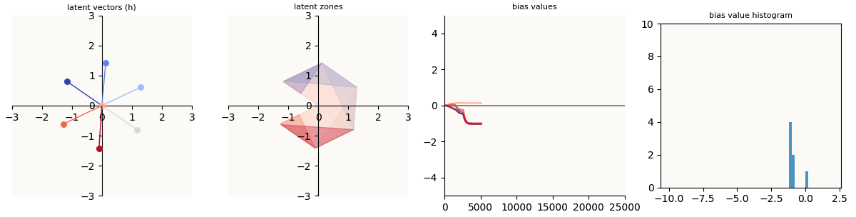
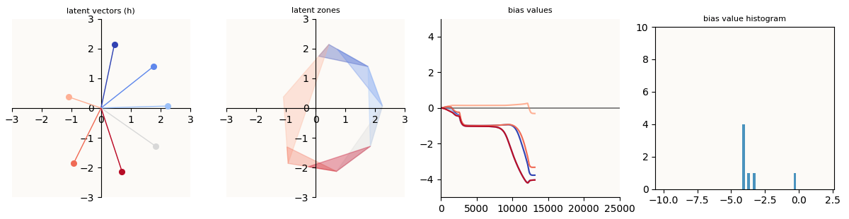
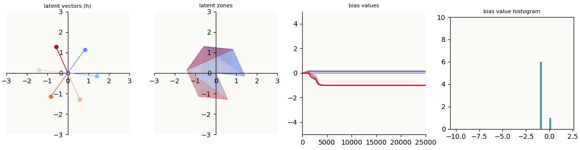n = 7, m = 2, trained for 25,000 epochs using AdamW

Symmetric Failure happens when the model fails to learn some / a feature (does not represent it at all), but does a perfect job of representing the rest (the other 6 features have equal magnitude and are spaced apart equally).

We now observe the pac-man shape as opposed to a regular hexagon. As explained above, because I draw the latent shape by simply connecting the 7 feature vectors, the unlearnt feature that is close to the origin causes there to be that pac-man mouth.

The key things to note are that:

For the features that were properly learnt (call them features $1$ to $6$), we see the characteristic activation sliver in the latent space.
For the feature (feature $7$) that was not properly learnt, that feature activates everywhere - the whole latent shape is blue. This is because this feature’s bias value is positive, causing the entire latent shape to have a positive value in the $7$-th dimension.
Observing the training process, the fact that this model’s internal features stayed like since about step 3,000 means that this is a local optimum.

We know what the perfect solution looks like. The latent shape should be a regular heptagon, and the bias should be such that it pushes the latent shape in the dense negative direction ($[-1, -1, …, -1]$). It should reside in the completely negative hyper-quadrant except for the 7 activation slivers that have positive values in their respective dimensions. In order to get from the current state of the Symmetric Failure model to this perfect solution, 2 things need to happen:

$b_7$ needs to decrease and eventually become negative - this pushes the entire latent shape down into the negative region of the $7$-th dimension (so that it will stop activating everywhere).
$W_7$ ($7$-th column of $W$) needs to become non-$0$ (and eventually take its own unique direction, but to learn a non-$0$ value is the first step) - this introduces a tilt (more on “tilt” later) in the latent shape such that only a sliver of the shape will be positive in the $7$-th dimension.

Why can’t the model do either of these? Let’s take begin to describe this local optimum and perturb it to see how strong of a local optimum this is.

It’s not AdamW’s fault: At some point, I suspected that AdamW may have been the culprit, because AdamW has weight decay, which is a form of regularization. I then trained the autoencoder using Adam without any regularization, but the same optimization failure occurred.

What is $b_7$? Why can’t it decrease?

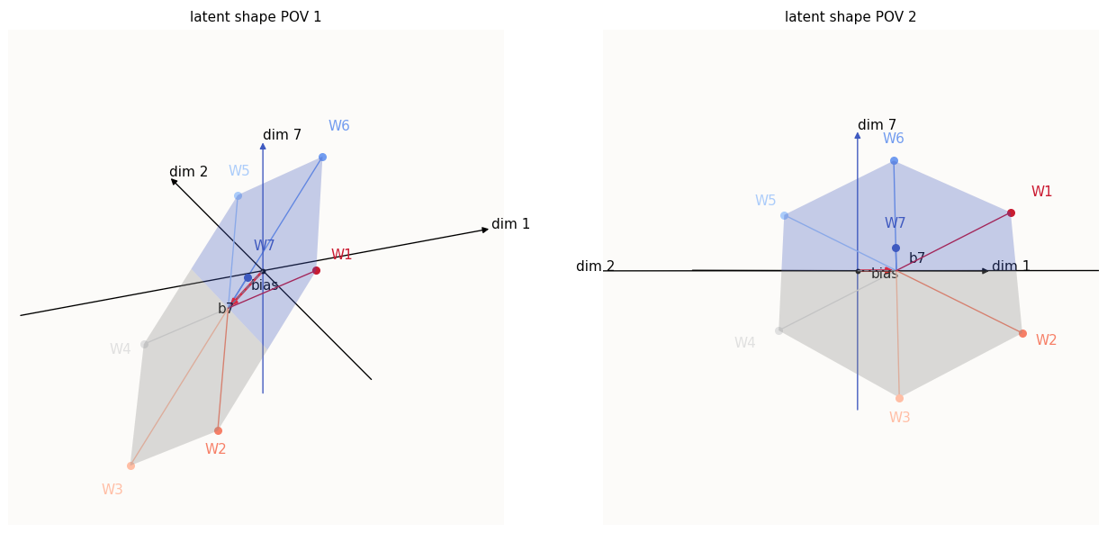
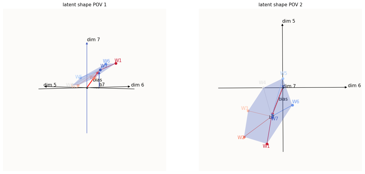
The first step is to solidify our intuition of $b_7$ and its relation to the position of the latent shape relative to the dim-$7$ axis, and of $W_7$ and its relation to the idea of “tilt”. This calls for more illustrations. Since I can’t illustrate in more than 3 dimensions, I’ll just illustrate in 3D. The nice thing about linear algebra is that the dimensions are all linearly independent, and we can just visualize any subset of dimensions without incurring some error from other dimensions. Hence, we’ll visualize our latent shape in dimensions 1, 2, and 7:

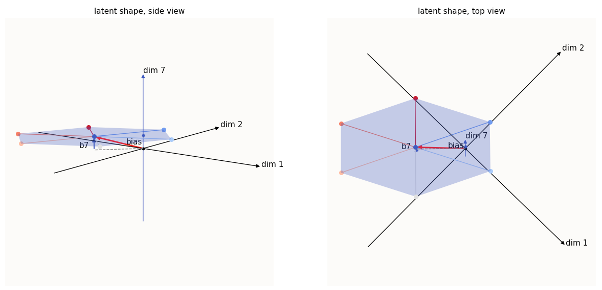The 1st, 2nd, and 7th dimension values of the latent shape (7-th dimension is enlarged)

I’ve drawn in the bias as well and highlighted $b_7$ (the value of the bias in the 7-th dimension). The entire hexagonal shape is also shaded blue to remind us that the entire shape is activated ($> 0$) in the 7-th dimension. You may notice that the hexagon seems squished - this is simply due to the fact that visualizing only 3 of the 7 dimensions results in this kind of “perspectival” squishing; the same thing happens when you try to take a purely side-profile look at a square piece of paper that’s half-tilted to face the sky - it doesn’t look square.

The important thing to note here is that $b_7$ is precisely the offset of the hexagonal plane with respect to the dim-$7$ axis. If you increase $b_7$, the plane moves up, and if you decrease it, the plane moves down.

Since $W_7 = 0$, the only thing that can impact the reconstruction of the 7-th feature is $b_7$:

\[\begin{align*} \hat{y} & = \text{ReLU} \left( W^\top W x + b\right) \\ \Longrightarrow \hat{y}_7 & = \text{ReLU} \left( W_7^\top W x + b_7 \right) \\ & = \text{ReLU} (b_7) \text{, because } W_7 = 0 \end{align*}\]

Remember that the model wants to be able to reconstruct a $1$ for the $7$-th feature of the $7$-th data sample, and a $0$ for the $7$-th feature of the other 6 data samples. If you had only 1 variable ($b_7$) to try and do this as well as possible, your best option is really to just encode the mean. And if your measure of error is Mean Square Error (MSE), then that the mean is really your solution. This is rather intuitive, and is also a standard result in Ordinary Least Squares (OLS) Regression because that also aims to minimize MSE. We expect $b_7 = 1/n = 1/7$ to hence be a local optimum, and from my experiments, it is indeed observed that $b_7 = 1/n = 1/7$.

What is $W_7$? Why can’t it increase?

In the perfect optimization case, $W_7$ is but one of the spokes of the feature wheel, and encodes the 7-th feature. In this case, it is $0$ and has failed to encode the 7-th feature. Turns out, this is also a local optimum; in this Symmetric Failure setup, $W_7$ prefers to remain $0$. To understand why this is so, we have to flesh out the idea of “tilt” that I briefly mentioned above.

Here, we go back to $W^\top W$ and compare how it should ideally look, versus how it looks like in this Symmetric Failure case:

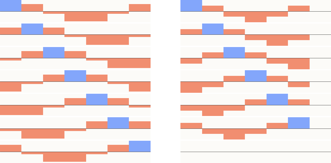Left: ideal W.T @ W (all 7 features learnt). Right: Symmetric Failure W.T @ W (only 6 features learnt)

The key observation is that the $7$-th row and column are $0$. This means that the latent shape (in the 7D reconstruction space) does not span the 7-th dimension. This means that the latent shape has no tilt with respect to the 7-th dimension.

Help: Do we call this the quotient space (Latent Plane / $e_7$)?

All of the $W_i$ introduce some tilt to the latent plane with respect to their own dimensions. If $W_7$ were to learn some non-zero value, it would introduce a tilt in the 7-th dimension. The simple way to see this is that if $W_7 \neq 0$, then the $7$-th row and column will be various non-$0$ values, which means that the plane given by $W^\top W$ will have some translation in the 7-th dimension, $\Longrightarrow$ tilt.

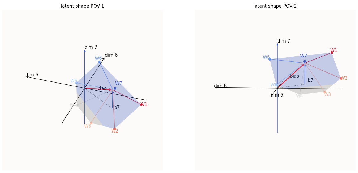
How tilt is generated

The first thing to note about creating tilt with $W_7$, is that the tilt will favor the $W_7$ direction. This means that the further along $W_7$ you go on the latent plane, the more positive the reconstructed value in the 7-th dimension gets. Simple math to sketch it out:

\[\begin{align*} \hat{y}_7 & = \text{ReLU} \left( W_7^\top W x + b_7 \right) \\ \end{align*}\]

Because $Wx$ is the hidden vector (i.e. “somewhere on the latent plane”), if $h = Wx$ has positive interference with $W_7$ (i.e. “along the positive $W_7$ direction”), $W_7^\top Wx$ will be positive. The more $h = Wx$ lies along the positive $W_7$ direction, the greater the value of $W_7^\top W x$, and the greater the value of $\hat{y}_7$.

Relatedly, the second thing to note is that the other features $W_i$ that lie on the same side of $W_7$ will also tilt towards a larger value in the 7-th dimension, while the other feathres $W_i$ on the other side of $W_7$ will tilt towards a smaller value in the 7-th dimension. To illustrate, let’s suppose $W_7$ is a mini version of $W_6$, i.e. $W_7$ $ = a \cdot $$W_6$ for small $a$:

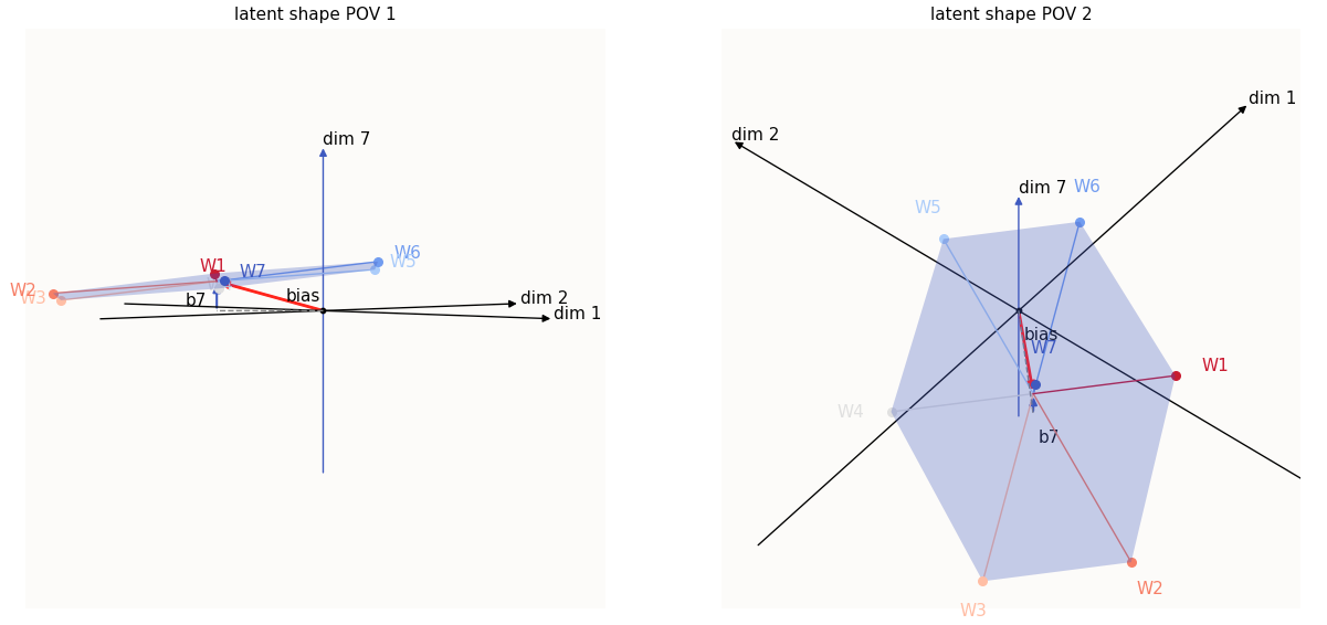Tilt introduced when W7 = 0.06 * W6

For a tiny value of $a = 0.06$, we introduced a tiny tilt to the latent hexagon. We limit the tilt such that the entire latent hexagon is still positive in dim-$7$, for our initial analysis. Both $W_7$ and $W_6$ are now tilting towards the positive direction along the dim-$7$ axis. To be more complete, features $W_5$, $W_6$, and $W_1$ are on the same side of the tilt as $W_7$ and are now more positive in the $7$-th dimension, while features $W_2$, $W_3$, and $W_4$ are on the other side of the tilt, and have less positive values in the $7$-th dimension.

Remember that correct value that we would like the model to reconstruct in the $7$-th dimension is $0$ for the first 6 data samples, because each of the first 6 data samples are not supposed to have an activated $7$-th feature. This means that because $W_5$, $W_6$, and $W_1$ now have a more positive value (further from $0$) in the $7$-th dimension, they are more WRONG, whereas because $W_2$, $W_3$, and $W_4$ now have values closer to $0$ in the $7$-th dimension, they are now more CORRECT.

You may think that there is symmetry here - the total additional error incurred (in terms of L2 distance) by the newly upward-tilted features is equal to the error reduced by the newly downward-tilted features - so the overall “correctness” of the untilted model and the tilted model is still the same, but this is not the case. What’s happening here is that because our loss (MSE) is convex (specifically quadratic), the additional error incurred by the upward-tilted features is larger than the error reduced by the newly downward-tilted features. We can sketch out a quick proof by looking at the loss changes incurred by $W_6$ and its mirror, $W_3$:

\[\begin{align*} \text{Old Loss} &= \text{Old Loss}_{W_6} + \text{Old Loss}_{W_3} \\ & = 2 b_7^2 \\ \text{New Loss} &= \text{New Loss}_{W_6} + \text{New Loss}_{W_3} \\ & = (b_7 + \Delta)^2 + (b_7 - \Delta)^2 \\ & = 2 b_7^2 + 2 \Delta^2 > 2 b_7^2 \end{align*}\]

This is simply Jensen’s Inequality at work. Again, convexity gives us the standard result of L2-regression (OLS regression) preferring mean values. The consequence: any tilt will incur more loss and the model will learn to correct it by preferring to set $W_7$ back to $0$. You can also calculate the gradients of the loss of each of the reconstructed data samples $\hat{y}^{(i \neq 7)}$ with respect to $W_7$ and observe that it will always point in the $W_7$ direction, which means that the update will be in the direction of $-W_7$.

When can the gradient favor more tilt after Symmetric Failure has happened?

In the previous section, we showed that by considering the other 6 features (i.e. $W_{i \neq 7}$), less tilt is always desired. However, we did not consider the error reduced by the newly learnt, non-$0$ value of $W_7$. In particular, we are interested to see if the error reduced for feature 7 can compensate for the overall increase in error for the other 6 features caused by the tilt, and if so, under what circumstances. Because if there are scenarios where it can compensate for the tilt - and of course there must be, how else can Perfect Optimization happen? - then we will have understood a mechanism for avoiding Symmetric Failure well. Be warned, a lot of this is just banging out the math.

[Skip to the last paragraph of this section (just before “Asymmetric Recovery”) if you don’t want to follow the dry math]

Let’s look at the gradient of the loss of the reconstruction of data sample $x_7$ w.r.t $W_7$:

\[\begin{align*} \frac{\partial \mathcal{L} (x_7)}{\partial W_7} & = \left( \hat{y}^{(7)} - y^{(7)}\right) \cdot \mathbb{1} \left\{ W^\top W x_7 + b > 0 \right\} \cdot \frac{\partial (W^\top W x_7 + b) }{\partial W_7} \\ & = \left( \hat{y}^{(7)} - y^{(7)}\right) \cdot \mathbb{1} \left\{ W^\top W_7 + b > 0 \right\} \cdot \frac{\partial (W^\top W_7 + b) }{\partial W_7} \text{, because } x_7 = e_7\\ & = \left( \hat{y}^{(7)} - y^{(7)}\right) \cdot \begin{bmatrix} 0 \\ 0 \\ \vdots \\ 0 \\ \vdots \\ 1 \end{bmatrix} \cdot \begin{bmatrix} \text{don't care} \\ \text{don't care} \\ \vdots \\ \text{don't care} \\ \vdots \\ \frac{\partial (W_7^\top W_7 + b_7) }{\partial W_7} \end{bmatrix} \text{, because the other 6 features don't activate} \\ & = \begin{bmatrix} \text{don't care} \\ \text{don't care} \\ \vdots \\ \text{don't care} \\ \vdots \\ \left( \text{ReLU} \left( W_7^\top W_7 + b_7\right) - 1\right) \end{bmatrix} \cdot \begin{bmatrix} \text{don't care} \\ \text{don't care} \\ \vdots \\ \text{don't care} \\ \vdots \\ 2W_7 \end{bmatrix} \\ & = 2 \left( \text{ReLU} \left( \|W_7\|_2^2 + b_7\right) - 1\right) \cdot W_7 \\ & = 2 \left( \|W_7\|_2^2 + b_7 - 1\right) \cdot W_7 \text{ (can drop ReLU as entire latent shape is > 0 in dim 7)} \end{align*} \\\]

And let’s also look at the gradient of the loss of the reconstruction of another data sample (not $x_7$), call it sample $x_j$ (where $j \neq 7$) w.r.t $W_7$:

\[\begin{align*} \frac{\partial \mathcal{L} (x_j)}{\partial W_7} & = \left( \hat{y}^{(j)} - y^{(j)}\right) \cdot \mathbb{1} \left\{ W^\top W x_j + b > 0 \right\} \cdot \frac{\partial (W^\top W x_j + b) }{\partial W_7} \\ & = \cdots \\ & = \left( \text{ReLU} \left( W_7^\top W_j + b_7\right) - 0\right) \cdot W_j \\ & = \left( W_7^\top W_j + b_7\right) \cdot W_j \text{ (likewise, can drop ReLU)} \end{align*}\]

The sum of these gradients from all 6 $x_{j \neq 7}$ is hence:

\[\begin{align*} \sum_{j \neq 7} \frac{\partial \mathcal{L} (x_j)}{\partial W_7} & = \sum_j \left( W_7^\top W_j + b_7\right) \cdot W_j \\ \end{align*}\]

There’s actually a rather neat way to simplify this, and it hinges on the fact that the features $W_{j \neq 7}$ are arranged in a symmetric fashion, where the $W_7$ line is the line of symmetry. This means that all the components of gradients that are orthogonal to the $W_7$ direction will all cancel each other out. For example, if $W_7$ is “front” to us, then the left-ward direction of $\frac{\mathcal{L} x_6}{W_7}$ will cancel out the right-ward direction of $\frac{\mathcal{L} x_1}{W_7}$. Likewise, the left-ward direction of $\frac{\mathcal{L} x_4}{W_7}$ will cancel out the right-ward direction of $\frac{\mathcal{L} x_2}{W_7}$. This means that we only have to consider the “front-back” ($W_7$) component of all these gradients, i.e. we can work with only the projections of these gradients onto $W_7$.

\[\begin{align*} \sum_{j \neq 7} \frac{\partial \mathcal{L} (x_j)}{\partial W_7} & = \sum_{j \neq 7} \left( W_7^\top W_j + b_7 \right) \cdot \hat{W}_7^\top W_j \cdot \hat{W}_7 \text{, by projecting } W_j \text{ to } W_7 \\ & = \sum_{j \neq 7} \left\{ \left(W_7^\top W_j\right) \cdot \hat{W}_7^\top W_j + b_7 \cdot \hat{W}_7^\top W_j \right\} \cdot \hat{W}_7 \\ & = \sum_{j \neq 7} \left \{ \|W_7\|_2 \left( \hat{W}_7^\top W_j\right)^2 + b_7 \cdot \hat{W}_7^\top W_j\right\} \cdot \hat{W_7} \\ & = \hat{W}_7 \cdot \sum_{j \neq 7} \left\{ \|W_7\|_2 \left( \hat{W}_7^\top W_j\right)^2 \right\} + \hat{W}_7 \cdot \sum_{j \neq 7} \left\{ b_7 \cdot \hat{W}_7^\top W_j\right\} \\ & = \hat{W}_7 \cdot \sum_{j \neq 7} \left\{ \|W_7\|_2 \left( \hat{W}_7^\top W_j\right)^2 \right\} \text{, because all } W_j \text{ cancel out} \\ & = W_7 \cdot \sum_{j \neq 7} \left( \hat{W}_7^\top W_j\right)^2 \end{align*}\]

I find this simplified form appallingly… simple; great because it significantly simplifies our calculations. So in order for us to favor tilt, the update has to be in the $W_7$ direction, which means the gradient has to be in the $-W_7$ direction, which means that:

\[\begin{align*} \frac{\partial \mathcal{L} (x_7)}{\partial W_7} + \sum_{j \neq 7} \frac{\partial \mathcal{L} (x_j)}{\partial W_7} & = (< 0) \cdot W_7 \\ 2 \left( \|W_7\|_2^2 + b_7 - 1\right) \cdot W_7 + W_7 \cdot \sum_{j \neq 7} \left( \hat{W}_7^\top W_j\right)^2 & = (< 0) \cdot W_7 \\ 2 \left( \|W_7\|_2^2 + b_7 - 1\right) + \sum_{j \neq 7} \left( \hat{W}_7^\top W_j\right)^2 & < 0 \\ 2 \left[ 1 - \left( \|W_7\|_2^2 + b_7 \right) \right] & > \sum_{j \neq 7} \left( \hat{W}_7^\top W_j\right)^2 \end{align*} \\\]

Without having to write out too much further math, we can see that this is impossible for any non-0 value of $W_7$. How? We simply observe that:

Both sides are quadratic in $W_7$, which means the overall shape of $LHS - RHS$ is also quadratic.
Since we are analyzing the regime where the entire latent hexagon is positive in dimension $7$, that also means that $b_7 > 0$. That means the maxmum value of $LHS$ is just $2$. In particular, to maximize the $LHS$, we want to minimize $|W_7|_2$, and to minimize the $RHS$, we also want to minimize $|W_7|_2$. Both sides will contribute optimization pressure to force $W_7$ to $0$.

What if Symmetric Failure and $b_7 = 0$?

Very briefly, we can extend our intuition from the previous section to make conclusions for the case of Symmetric Failure and $b_7 = 0$. Most notably, this means that the latent hexagon is pivoted on the dim-$7 = 0$ hyperplane, such that if there is a tilt, half of the latent hexagon will tilt upwards, while the other half will tilt under dim-$7 = 0$.

Tilted latent hexagon at b7 = 0

This is significant because the half that is in the negative region (in dim-$7$) will be “deactivated” by ReLU (i.e. set to $0$). This impacts $\mathcal{L}(x_{j \neq 7})$, where $j$ are the indices of the features that are negative in dim-$7$, because they are now $0$. This means that the model now has no loss for samples $x_2$, $x_3$, and $x_4$, hence these samples no longer exert any optimization pressure to “untilt” the latent hexagon, but the other samples still exert that same untilting optimization pressure. The above calculation will still hold, just that there are now only half the number of $W_j$’s.

So now, we conclude that when $b_7 \geq 0$ and we’re in the Symmetric Failure case, we’re stuck. Constrained to $b_7 \geq 0$, this is the best we can do.

Asymmetric Recovery

We have since found that once we’ve reached Symmetric Failure, assuming that the learnt $W_i$’s are all symmetric (equal magnitude and equally spaced apart in a circle), and $b_\text{unlearnt} \geq 0$, we’re kind of stuck. Let’s move on to the next mode of behavior and see what happens when the symmetric constraint on $W_i$’s is broken, and how that might happen in the first place.

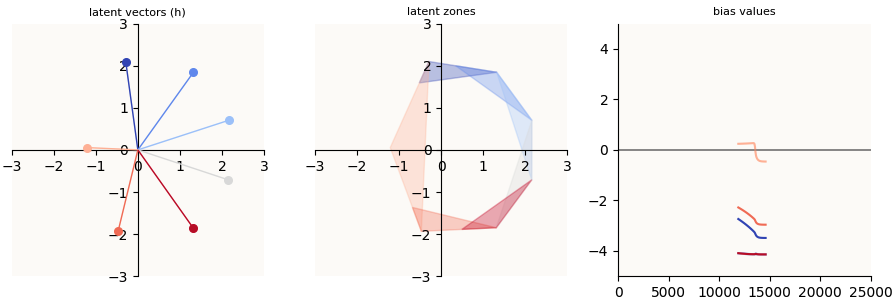
To quickly describe, Asymmetric Recovery happens when we reach Symmetric Failure, but at some point, the $W_\text{learnt}$’s begin to skew such that one side has much larger features than the other, the $b_\text{learnt}$’s begin to become much more negative, and then $W_\text{unlearnt}$ and $b_\text{learnt}$ finally get learnt, achieving a 0-loss model.

Symmetric Failure Reached

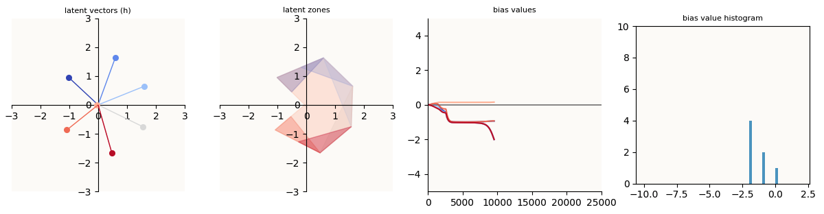Skew begins to show

W7 increasing and b7 decreasing

Asymmetric Recovery achieved

Note that the color mappings between these ‘training progress’ plots and the latent visualization plots are different, simply because I can’t tell ahead of time (without excessively more code to write) which feature will be the unlearnt feature, and hence which feature to color dark blue.

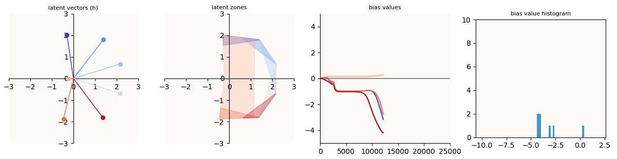
Let’s try to make sense of what’s going on at the skew stage. The skew stage is characterized by elongating learnt feature vectors $W_\text{learnt}$ as well as $b_\text{learnt}$ values that get increasingly negative (except for the initial increase for a number of that). The fact that these 2 behaviors happen simultaneously makes sense to me.

Skew stage

If you look at the right view of the latent shape, you can realize that, for example, as $b_5$ gets increasingly negative, the latent shape will shift in the negative direction in dim-$5$. This means that to preserve the activation sliver for feature $5$, $W_5$ has to be longer such that it can still reach the positive region in dim-$5$.

Remember that the goal of the reconstruction of each feature is to have the model output a $1$ whenever that feature is supposed to be active. This affects the extent to which $W_i$ must protrude into the positive region of dim-$i$, because:

\[y_i = \text{ReLU} (W_i^\top W_i - b_i)\]

Because $b_6$ and $b_1$ are less negative (smaller magnitude), $W_6$ and $W_1$ are also shorter. This asymmetry is important because it actually helps us favor the forces that generate the tilt in dim-$7$. Remember that the sum of all the data sample errors w.r.t to $W_7$ is:

\[\begin{align*} \sum_{j \neq 7} \frac{\partial \mathcal{L} (x_j)}{\partial W_7} & = \sum_j \left( W_7^\top W_j + b_7\right) \cdot W_j \\ \end{align*}\]

In the Symmetric Failure case, we could appeal to arguments of symmetry to say that the total uptilt introduced is equal to the total downtilt introduced, but because of convexity, bla-bla-bla, the total gradient points in the $W_7$ direction, which makes the update favor untilting. However, now, the vectors on the opposite side of $W_7$ (negative $W_7^\top W_j$) are significantly longer than those on the same side of $W_7$ (positive $W_7^\top W_j$). This overcomes the tendency towards untilting induced by the convexity of MSE, and allows the total gradient to point in the $-W_7$ direction, and for the update to favor tilting! Another way of phrasing is that the imbalance of the learnt vectors causes the local optimum of $W_7$ to shift away from $0$. This imbalance, where the originally learnt features get longer, is what makes it possible for $W_7$ to eventually get learnt. In other words, $W_7$ only gets learnt because the original set of features “graduated” to a higher radius! After encountering “Symmetric Failure,” having features split into “circles” of multiple radii is desirable!

At some point, the plane tilts so much that some of the features $W_{j \neq 7}$ begin to dip into the negative dim-$7$ region. This means that the loss incurred by those corresponding data samples become $0$.

Some features (W3, W4) achieve 0 loss in dim-7

This is not convenient for us because we have fewer contributors to the tilting force. At some point, all the learnt features $W_{j \neq 7}$ on the other side of $W_7$ (i.e. negative dot product with $W_7$) will be in the negative dim-$7$ region, generating no more loss. The only features generating loss left will be the features on the same side of $W_7$ ($W_6$, $W_1$), and $W_7$ itself. Except for $W_7$, the other features will generate an untilting force, which will easily outweigh the tilting force generated by $W_7$. This initially seemed like it would be a problem, but turns out, by the time this would happen, $W_7$ would already have such significant magnitude that the added performance of being able to encode the $7$-th feature would outweigh the slight increase in loss of the features $6$ and $1$.

How does one side magically start to elongate?

If we consider only the 6 learnt features, we have already achieved a 0-loss solution; the 6 features are equally spaced out on a wheel, and have more or less the same magnitude. The fact that there is a “skew” that is being introduced, and that the skew always “sweeps” the learnt feature vectors to the opposite side of the unlearnt feature ($W_7$), can only mean that this is due to either $W_7$ or $b_7$.

Small asymmetry in Symmetric Failure?

It is a fact that the 6 learnt features are never truly symmetric, because gradient descent is a numerical method; it is merely almost exactly symmetric. Some learnt features are slightly shorter than others, but the model can compensate by adjusting the biases and the angles between the features accordingly to compensate. Let’s look at how this happens by deliberately introducing some asymmetry.

Suppose we introduce a perturbation such that $W_6$ and $W_1$ are now both a tiny bit shorter than the other $W_{j \neq 7}$. Now we’ll have some loss, because the activations for features $6$ and $1$ are not as strong, and there’s interference. This triggers a series of updates that will cascade the loss from one side (the side of $W_6$ and $W_1$) the other side of the latent space:

Because of insufficient activation of features $6$ and $1$, the model would update itself and try to elongate $W_6$ and $W_1$ and decrease $b_6$ and $b_1$.
Because features $6$ and $1$ are also now interfering with each other, the update will also want to push $W_6$ and $W_1$ away from each other.
This causes features $6$ and $1$ to now interfere with features features $5$ and $2$ respectively, so the same updates of pushing $W_5$ and $W_2$ away (move to the right side) and outward (elongate) will happen.
By the same mechanism, these updates will cascade all the way to all the features on the opposite of the latent space.

Pictorially:

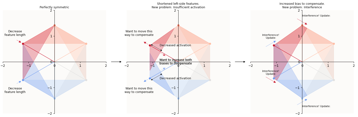Constructing a slightly asymmetric, 0 loss solution

This type of “skewing” of the feature vectors towards one side would also happen if instead of $W_6$ and $W_1$ being slightly shorter, $b_6$ and $b_1$ were more positive (because the same effects of insufficient activation and interference would happen). Here’s one such “slightly asymmetric” solution - notice how the feature vectors seem to be more splayed out on the left side, and more elongated on the right side, as if there’s a repulsor on the left and an attractor on the right:

One such slightly asymmetric, 0 loss solution

We’ve now observed that any small perturbation in weights near the Symmetric Failure scenario results a series of small updates (skewing features to one side) to quickly re-establish 0 loss. This is how the model compensates for small asymmetries to arrive at a new loss-less equilibrium. Though it’s great that the model can recover like this, there’s unfortunately no “run-away” or self-reinforcing mechanism that would cause the skewing action to keep happening to the extent that it does in “Asymmetric Recovery” - what gives?

Small asymmetry favoring tilt

In the previous section, we examined what happens if there are small asymmetries in the learnt features, and we considered only the learnt features and their corresponding training data samples. However, if we added the unlearnt vector back in, we find that this generates the run-away sweeping effect we are looking for! Let’s start with a Symmetric Failure (with the above subtle asymmetry) set of weights. Note that:

$W_6$ and $W_1$ are ever so SLIGHTLY shorter, and correspondingly, $b_6$ and $b_1$ are more positive (around $\approx -0.988$, while the rest are $-1.02 \sim -1.03$).
$W_2$ and $W_5$ are now tilted SLIGHTLY to the right side (important!)
This set of weights has $\approx 0$ loss on the 6 examples for which the learnt features correspond to.

Example ‘Symmetric Failure’ with some asymmetry

The first thing to note that having asymmetry in the 6 learnt vectors induces a new optimum on $W_7$ that is not $0$ anymore. Previously, when the 6 learnt vectors formed a perfectly symmetric hexagon, we could say: if the latent hexagon tilted one way, half of the predictions will have a larger value ($\approx \frac{1}{7} + \Delta$) for the $7$-th logit, while half of the predictions will have a smaller value ($\approx \frac{1}{7} - \Delta$), but since loss (MSE) is convex, the additional loss incurred by the larger values will outweigh the loss savings of the smaller values, hence the system will want to remove tilt.

In this case, notice that:

There are more vectors on 1 side ($W_2$, $W_3$, $W_4$, $W_5$) than the other ($W_6$, $W_1$). So, if the tilt is such that the more populous side moves down in dim-$7$, there are more contributors to the loss savings.
The vectors on the left side ($W_6$, $W_1$) are shorter, which means that the $\Delta$ along dim-$7$ incurred by the tilt on each of these 2 vectors is going to be slightly less than those of their opposite vectors.

These two factors contribute to the loss having a local optimum at $W_7 = \varepsilon \cdot (W_6 + W_1)$, i.e. still very near $0$, but shifted somewhere in the $W_6$ and $W_1$ direction. I empirically confirmed this by freezing all the learnt weights and letting $W_7$ settle at its local optimum.

The second to note is that having a non-zero $W_7$ now means that the learnt vectors will also want to update in the opposite side of $W_7$:

\[\begin{align*} \frac{\partial \mathcal{L}(x_7)}{\delta W_{j \neq 7}} & = (y_7 - x_7) \cdot \mathbb{1} \left\{ W^\top W_j + b > 0 \right\} \cdot \frac{\partial (W^\top W_j + b) }{\partial W_j} \\ & = \begin{bmatrix} 0 \\ 0 \\ \vdots \\ 0 \\ \vdots \\ W^\top_7 W_j + b_7 \end{bmatrix} \cdot \begin{bmatrix} \text{don't care} \\ \text{don't care} \\ \vdots \\ \text{don't care} \\ \vdots \\ \frac{\partial (W_7^\top W_j + b_7) }{\partial W_j} \end{bmatrix} \text{ (the other 6 features are correctly reconstructed)} \\ &= (W_7^\top W_j + b_7) \cdot W_7 \end{align*}\]

This means that there are 3 forces at play (first 2 described in previous section):

(Due to asymmetry of learnt vectors) insufficient activation for learnt features (updates will favor elongating feature vectors)
(Due to asymmetry of learnt vectors) inteference between learnt features (updates will favor splaying out and sweeping vectors to one side)
(Due to $W_7 \neq 0$) all other features will update in favor of the $-W_7$ direction (i.e. also sweep towards $-W_7$) I’ve illustrated what the weight updates look like when we start from this set of weights:

The lengths of the updates can be misleading since I’ve normalized them such that the biggest update has magnitude 1. In particular, it is not that the updates (learning_rate * - gradient) of $W_{j \neq 7}$ are getting larger, but that the dominant update ($W_7$) is decreasing very rapidly, so the others look like they are increasing rapidly in comparison.

We know that the first 2 forces will result in a small amount of splaying / sweeping, but because this splaying / sweeping creates an imbalance (the opposite side of $W_7$ is now more populous and longer), this shifts the local optimum of $W_7$ even more towards the positive $W_7$ direction. This means that the third force, which is function of $W_7$, will increase (since $W_7$ is now larger). This causes more sweep, which shifts the local optimum of $W_7$ yet again, so on and so forth. This, is the run-away tilting effect we are looking for. Eventually, the skew in vectors is so large that the local optimum for $W_7$ basically becomes so positive that it over-activates the $7$-th logit and causes $b_7$ to very quickly decrease into being negative, achieving no loss on all data samples (Asymmetric Recovery).

Asymmetric Recovery Achieved (color coding of vectors is different)

Asymmetric Recovery is Chaotic

The real kicker here is that this sort of recovery can happen not only in the subtly asymmetric case, but in the Symmetric Failure case as well - after all, the probability that the 6 learnt vectors ($W_{j \neq 7}$) in the Symmetric Failure case are perfectly symmetric is $0$. so there is always some subtle asymmetry. In reality, because our learning algorithm (gradient descent) is iterative, this recovery doesn’t happen very much though, because it relies on the learning rate and the specific configuration of asymmetry (which vectors are too long / short, by how much, etc.) to be in a sweet spot. The closer you are to perfect Symmetry Failure, the more susceptible asymmetric recoverability is to chaotic behavior (critical), because gradient descent steps are very likely to change the confluence of factors that give rise to the above 3 forces. Perhaps you took too large a step and now $W_7$ has flipped direction, causing the third force to also flip, or perhaps an update to $W_6$ and $W_1$ pushed them outwards too far and the local optimum for $W_7$ gets set closer to $0$. Perhaps the asymmetry wasn’t so fortuitous to begin with (e.g. $W_{j \neq 7}$ were alternatingly short and long). This explains why Asymmetric Recovery is very rare (anecdotally, I trained 100 randomly seeded such auto-encoders and only got 1).

In fact, this is general. Knowing whether a model is going to exhibit some behavior (converge, diverge, achieve Asymmetric Recovery) is in general hard to predict for iterative algorithms. I found this blogpost / preprint by Jascha Sohl-Dickstein on the fractality of neural network training (when plotting whether training converges vs diverges over learning rates) to make a lot of sense. His illustrations of the chaotic patterns (it seems more merely chaotic than fractal to me) are particularly relevant to what’s going on here. (And of course, I later discovered that he works at Anthropic… another reason to love their research).

The reason I focused on this special case of having 2 adjacent features perturbed is that this is basically rigging the weights such that asymmetries line up with each other (perturbed features are on the same side, and also the same side as $W_7$). It hence offers a good shot of achieving Asymmetric Failure (it is not too near critical points).

And because seeing is believing, to see the chaotic behavior in our case, we can construct a similar plot of how much splaying / sweeping happens (I’m most interested in this phenomenon because it is a crucial prerequisite to Asymmetric Recovery) over 2 variables: the magnitude of the perturbation to both $b_6$ and $b_1$, and learning rate. The sum of the magnitudes of all the $W_j$ are the metric I plot here as a measure of how much splaying / sweeping there is:

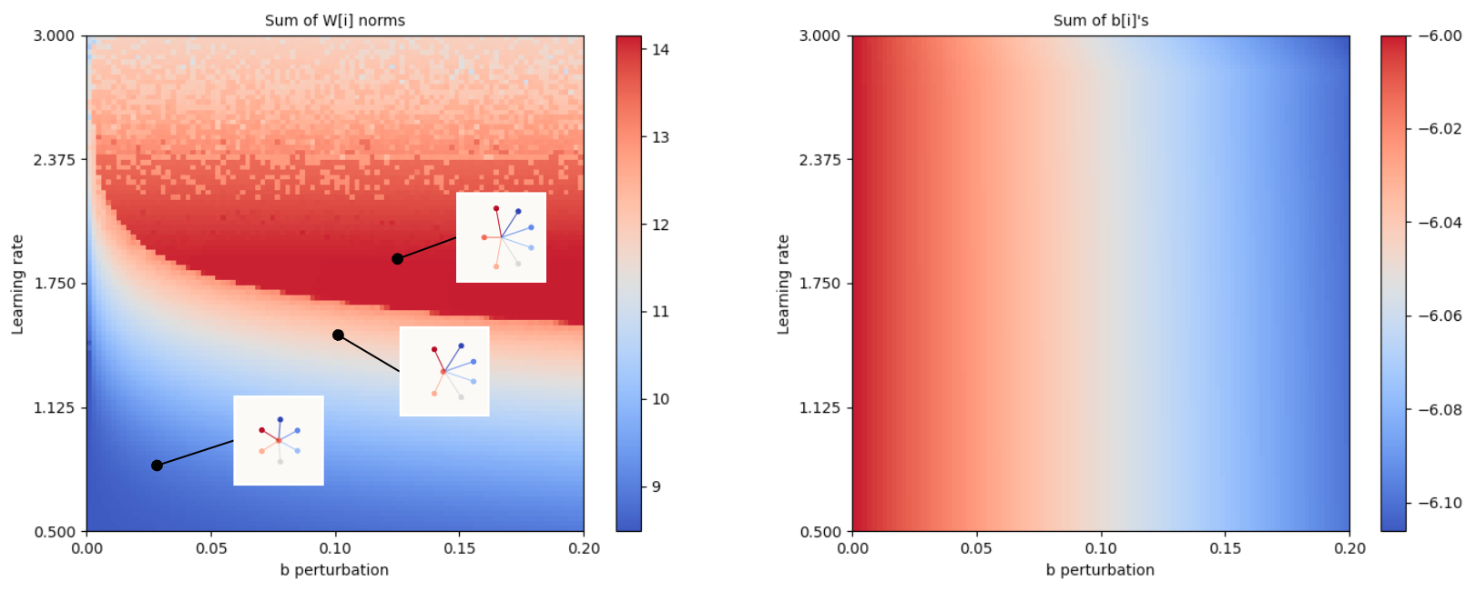Interpret this as ‘how much splay / sweep occurs with a certain perturbation introduced to b6 & b1 and at a certain learning rate?’

We notice two things from this plot:

The amount of splaying / sweeping generally increases with learning rate, but starts to get patchy beyond a certain point. This indicates that the ability of a model to achieve splaying / sweeping / Asymmetric Recovery isn’t just a question of whether there’s a sufficiently high learning rate, but rather, if the learning rate in a sweet spot that depends on all other factors (which features are too long / short, which biases are too large / small, by how much, and so on). This demonstrates the chaotic behavior that we postulate. I’d like to point out, though, that this seems like very much equivalent to how doing standard Stochastic Gradient Descent (SGD) on a simple convex surface can either converge (learning rate is sufficiently small) or diverge (learning rate too large); in this case, perhaps our problem isn’t chaotic, but that it’s so complex that it effectively requires us to search over an exponential combination of factors - not chaotic, but impractical.
At a fixed amount of perturbation to $b_6$ and $b_1$, the amount of splaying / sweeping is a function of learning rate. Notice also that at basically 0 perturbation to $b_6$ and $b_1$, we still see some amount of splaying / sweeping. This reiterates just how much influence SGD has on optimization failure as an iterative algorithm.

Bringing It All Together

So far, we have:

Illustrated what the latent space of our model looks like, and how there are latent zones, the sizes of which are determined by the need to have “sufficient activation / reconstruction”, which
Answers the question of what is meant by “Optimization pursues linear separability,” and answers the question of why shorter features need to be more widely spaced apart.
Understood why Optimization Failure (Symmetric Failure) happens - the local optimality of Symmetric Failure - but that
Small fortuitous asymmetries can cause a runaway splaying / sweeping of learnt features to happen, which is a prerequisite for Asymmetric Recovery,
which happens when there is so much splaying / sweeping that the local optimum for the unlearnt feature is sufficiently far away from $0$ that it’s basically “learnt”

Avoiding / Correcting Optimization Failure

So then, what next? The ideal next step is obviously to prevent Optimization Failure altogether, but seeing that this phenomenon is chaotic (or at least “non-polynomially complex”), this is basically impossible. The best we can do is to reason probabilistically about the best conditions that we can try to create to avoid or correct Optimization Failure, and this, Anthropic has basically begun to do. In this next section, I will examine their neuron resampling method to see how well they work, how we may reason theoretically about it, and if we can do better.

Anthropic’s Resampling Procedure

I’ll try my best to accurately summarize what Anthropic’s resampling method is, which is difficult because of the confusion between the terms “dictionary vector” and “encoder vector,” which they do not define explicitly.

First, let’s look at their sparse auto-encoder:

\[\begin{align*} \bar{x} & = x - b_d\\ f & = \text{ReLU}(W_e \bar{x} + b_e) \\ \hat{x} & = W_d f + b_d \\ \end{align*}\]

This is very similar to the toy ReLU auto-encoder that we investigated in the post. In particular:

$W_e$ is a tall matrix (the SAE has more features than the width of the inputs $x$), and is enclosed by ReLU, which is the same mechanism that gives us “free” dimensions as in the auto-encoder - a projection to a higher-dimensional space followed by $\text{ReLU}$.
Just like how our toy ReLU auto-encoder wants to reconstruct the input, so does this SAE.

I’ll then lay out the assumption (inferred from their blogpost) that:

“Dictionary vector” refers to one column of $W_d$
“Encoder vector” refers to one row of $W_e$

And this is their resampling procedure. After some number of training steps, they:

Compute the loss of the current SAE on a random sample of 819,200 $x$’s.
Assign each $x$ a probability of getting selected that is proportional to the square of their loss $\mathcal{L}(x)^2$.
Identify neurons (you can think of a neuron $i$ as the $i$-th row of $W_e$, or the $i$-th column of $W_d$, or the SAE feature vector $(W_e)_i x$) that are dead ($(W_e)_i x = 0$) for the last however arbitrarily many samples of $x$. For each of these dead neurons, call neuron $i$:
1. Sample an input according to the probabilities computed in step (2) - i.e., preferentially sample the $x$’s on which the SAE does badly on.
2. Decoder / dictionary: Normalize the sampled $x$ to get $x_u$, such that $x_u$ has magnitude 1, and set $(W_d)_i = x_u$
3. Encoder: Renormalize $x$ to get $x_s$, such that $x_s$ such that $|x_s| = 0.2 \times \frac{1}{\text{num alive}} \sum_{j}^{\text{num alive}} |(W_e)_j|$, and set $(W_e)_i = x_s$.
4. Set $(b_e)_i = 0$.
5. Reset Adam optimizer parameters for every modified weight and bias to 0.

They claim that “Resetting the encoder norm and bias are crucial to ensuring this resampled neuron will only fire weakly for inputs similar to the one used for its reinitialization.”

Why it works

For openers, let’s emphasize that this neuron resampling method does not put the neuron’s weights in an “ideal” state, as if hand-picking the weights to magically transform Asymmetric Failure to Perfect Symmetry. Training cycles still have to happen after in order to let the model adjust the changed weights and achieve a new, presumably better, optimum.

With that out of the way, we note how the above resampling procedure changes the model.

Neuron $i$ is Alive

Inputs similar to the one used for neuron $i$’s reinitialization, call $x$, will now no longer be dead. Simply put:

\[\begin{align*} f_i & = (W_e)_i \bar{x} + 0 > 0 \\ \hat{x} & = W_d f + b_d \\ & = (W_d)_i f_i + \sum_{j \neq i} (W_d)_j f_j \end{align*}\]

Notice how $f_i > 0$, meaning that the neuron is now firing (no longer dead). And $\hat{x}$ is now closer to $x$. We can observe this by noticing that only the terms ($(W_d)_i, (W_e)_i$) interacting with $f_i$ has changed, and if $(W_d)_i$ is colinear with $x$, which it is, then whereas $(W_d)_i f_i$ used to be $0$, it is now some small multiple of $x$, i.e. closer to $x$. This argument holds true if either $(W_d)_i$ or $(W_e)_i$ is a small multiple of $x$, because otherwise the new $\hat{x}$ could be so large that it is further from $x$ than $0$ is from $x$, which explains the arbitrary $0.2$ multiplier applied in setting $(W_d)_i$.

In my explanation, I assumed that $\bar{x}$ is “close” to $x$, that I used them interchangeably. In reality, they are probably not that close, and I do not know which one Anthropic is referring to when they say “input vector.” I suspect even though $\bar{x}$ and $x$ are not close, the relationship between $\bar{x}$ and $x$ (the shift by $-b_e$) will resemble the relationship between the various $W_i$’s and $b$ in this post, and that there will still be positive dot-product between $\bar{x}$ and $x$, which allows my explanation to still apply.

Interference is Introduced

Because this procedure magically just assigned $(W_e)_i$ to encode a feature similar to $x$, just like how each $W_i$ are assigned to each input feature in this post, there is nothing stopping $(W_e)_i$ from interfering with any number of other rows of $W_e$. In the context of this post, this will look as if we just introduced a full-length $W_7$ between $W_6$ and $W_1$ such that $W_7$ is now in $W_6$’s and $W_1$’s latent zones. This will cause the model to adjust in the following ways in the next few iterations:

The rows that $(W_e)_i$ now interferes with splay apart and sweep to other side to reduce interference
$(W_e)_i$ itself causes the other features that interfere with it to over-activate and incur more loss, hence the model would want to decrease $(W_e)_i$ to counteract this added loss (this is the “untilting” force in this post)
Depending on the value of the new $f_i$, $(b_e)_i$ could have a gradient in either direction

Because the relationship between these forces are quantitatively hard to pin down (there’s also learning rate in this mix of factors!), we don’t know for sure (or even probabilistically) if the model is going to:

Push $(W_e)_i$ back to its local optimum (which is presumably still near $0$)
Cause the other rows of $W_e$ to splay and sweep and eventually favor a new local optimum for $(W_e)_i$ that would be functionally equivalent to having learnt a new feature ($x$)

This seems to me to be a clumsy solution. For sure, option (2) is possible, and if you keep resampling enough, you will definitely learn more and more features, which is why the method achieves positive outcomes. However, I think a much more elegant solution is to introduce an overall asymmetry to the rows of $W$ the way we perturbed the biases in this post.

A Possible New Method

In this post, we perturbed the biases $b$ corresponding to features ($W_i$) on the same side of the latent space, in the same direction ($+\Delta$ for both). This introduced a very consistent direction of asymmetry into the model’s internal features ($W, b$). We also saw that despite the recovery behavior being chaotic, there still exists regions (combinations of $\Delta$ and learning_rate) where recovery is overwhelmingly likely, and regions where it is not. We also saw that recovery happened without us having to assign any direction to $W_7$ in the sense of explicitly mapping $W_7$ to any input.

This seems to suggest that so long as we can arbitrarily define a repulsor (a direction that features will splay apart or away from) and an attractor (a direction that features will sweep towards), where the repulsor and attractor are colinear but in opposite directions, and seed all the dead neurons (the equivalents of $W_7$) to be ever so slightly positive in the repulsor direction (with some tiny tiny numerical noise to differentiate them), and positively perturb all the biases whose corresponding neurons (rows of $W_e$) have a positive dot-product with the repulsor, the model will likely splay / sweep all the live neurons apart and recover all the dead features that exist, without us having to do any of paired mappings over $((W_e)_i, (W_d)_i)$ and $x$’s.

Explicitly, I hypothesize that this following resampling method will work well:

Compute the sum of all live neurons $\Sigma = (W_e)_j$. Normalize $\Sigma$ to have magnitude 1. The attractor direction will be $\Sigma$ and the repulsor direction will be $-\Sigma$.
Set all dead neurons $ (W_{e})_{i} $ to be some small fraction of the average magnitude of all the live neurons: $\begin{align*} (W_{e})_{i} = 0.05 \times -\Sigma \times \frac{1}{\text{num alive}} \sum_{j}^{\text{alive}} \|(W_e)_j\| + \varepsilon \text{, where } \varepsilon \sim \mathcal{N}(0, \text{very small}) \end{align*}$
Positively perturb bias entries whose corresponding neurons are on same side of repulsor: $\begin{align*} (b_e)_j \longrightarrow (b_e)_j + \Delta, \forall j \mid (W_e)_j \cdot -\Sigma > 0 \end{align*}$

This is better because:

It doesn’t require us to do any of paired mappings over $((W_e)_i, (W_d)_i)$ and $x$’s.
We have an understanding that there exist regions of high probability of success, and a simple parameter sweep across $\Delta$ and learning_rate will allow us to confidently choose good values for them.
The choice of which features ($x$’s) to recover will not be left to chance - they will be automatically recovered so long as they are “important enough” or mistakes on them are “costly enough,” which mimics Anthropic’s mechanism of assigning a selection probability to each $x$ that is proportional to their reconstruction loss.

Overall, it seems like a more elegant solution, and worth experimenting with. I will, however, not be conducting this experiment in the near future as it’s quite a bit of work and I’m at the moment more drawn to the mysterious behaviors of Feature Splitting and Feature Absorption in SAEs. This is something that I would love to pick back up if anyone would like to be collaborators to work with me though!

Closing Words

Surely, this is a kind of investigation that nobody has done or taken the time to pen out, and I hope that if nothing else, you at least got a visual glimpse / intuition into what the latent space of a ReLU model looks like. I think this is the sort of intuition that is very necessary to try at further interpretability problems involving features and optimization pressures that cause features to form or fail to form.

I also wish that I had a comments section so that there could be some feedback, but that is also, quite a bit of work. If you’ve engaged with this post all the way to the end, I’d love to hear what you think - send me an email! 🙂

Optimization Failure