This post is the prequel of the next post, “Optimization Failure”, where I investigate how, even in cases where perfectly symmetric, ideal weight configurations exist, ReLU toy models (following Anthropic’s setup) may still end up with asymmetric solutions, termed as “Optimization Failure”.
Introduction
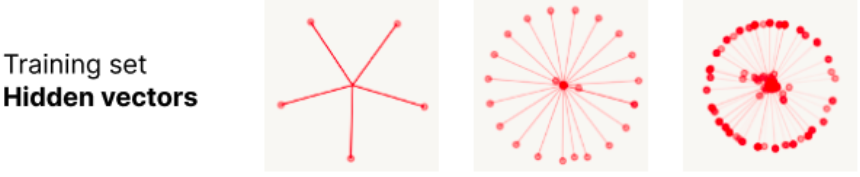
It grew pretty obvious while working on “Optimization Failure” that having an excellent geometric intuition of the feature space in ReLU Toy Models was crucial. Until recently, deep models were considered black boxes; needless to say, people didn’t really thinking about mapping out latent spaces of models. However, the latent spaces of models that use ReLU as their activation function are surprisingly intuitive. There’s a general rule of thumb that all features are generally linear. By that, I mean that each feature has its own direction in latent space. Sometimes, you see multiple features that relate to each other in non-linear ways - for example, the features representing each day of the week were found to be arranged in a circle (Engels et. al), but even then, the individual features of each day of the week have their own direction.
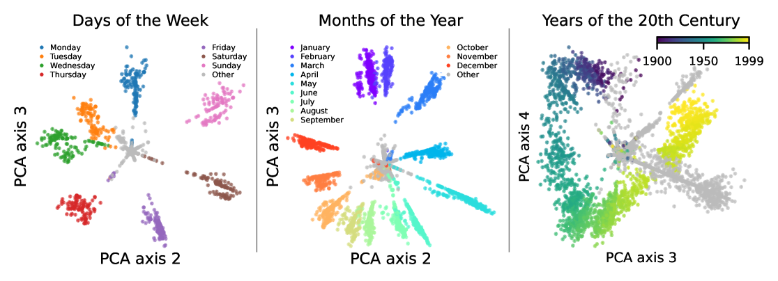 Features recovered by Engels et. al
Another key feature of latent spaces is the superposition of features. This refers to a large number of features embedded in a relatively low-dimensional space (the number of dimensions is lower than the number of features), necessarily leading to features having to share dimensions and be non-orthogonal. In the above example, you can see that features are spaced less than 90 degrees apart from each other. A more rigorous way to describe this that makes their non-orthogonality clear is that multiple features have some degree of colinearity. This is a simple consequence of trying to project a large number of dimensions (1 dimension = 1 feature) onto a smaller dimensional space, and unless you have some way to disambiguate each of the original dimensions from each other in the lower-dimensional latent space, you will have “interference”. Interference is undesirable because of information loss - given a latent representation of Friday, how would you know if the original data-point was truly a Friday, or a Thursday plus a Saturday? This picture from Anthropic’s Monosemanticity Paper explains it quite nicely:
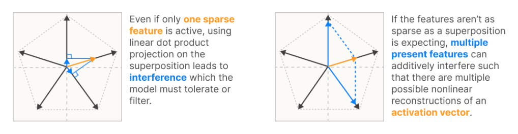 We don’t know if a feature is truly that single feature or a combination of multiple
Despite this, ReLU models can still reconstruct these features with very little error, which means that they are successfully avoiding the problem of intereference.
This post aims to make the geometric intuition very clear. We will go over the mathematical components of the ReLU model, demonstrate how each component contributes to the model’s ability to superpose features in its latent space without running into interference. With this geometric intuition, it will also become exceedingly clear why many features are generally “linear” in ReLU models.
Problem Setup
All deep models perform some sort of information compression; it is how models learn generalizable features, instead of memorize individual data points. This is not a question; it is a fact, and there are many papers on Grokking and Memorization that discuss this. It thus makes sense that Anthropic decided to study a small, toy version of a compression model that aims to take in a high-dimensional input, compress it into a small-dimensional latent, and decompresses it to try and reconstruct the input. A strictly linear model would find this impossible, but throw in a non-linearity (ReLU), and this becomes possible.
Anthropic’s Problem Set-Up
Given a high-dimensional input $x$, they train an auto-encoder to reconstruct $x$ (call the reconstruction $y$), by doing the following:
\[\begin{align*} y & = \text{ReLU}\left(W^\top W x + b\right) \\ \end{align*}\]Where $x \in \mathbb{R}^n, W \in \mathbb{R}^{m \times n}$. $n$ refers to the data’s dimensionality (input dimensionality) and is much higher than $m$, which is the latent dimensionality (aka “hidden dimensionality”).
There is also a sparsity level of $S = \text{around } 0.999$, which means that every entry of each data sample has a $0.999$ chance of being $0$, and being uniformly sampled from $(0, 1]$ otherwise. After sampling, these data vectors are normalized to have magnitude 1.
My Problem Set-up
We stick to the same toy model, but focus on the case of $n > 2, m = 2$. We will not have a sparsity parameter, but simply have all data samples be perfectly sparse (1-hot) vectors. This is because, while Anthropic was investigating the effect of sparsity on whether or not the model would eventually learn to superpose features or drop features that it had no capacity to express, I want to simply focus on the case where we know that a solution that perfectly superposes all features is possible. This is exactly the case where all input features are perfectly sparse (each data sample has only 1 feature active); this is corroborated by the fact that Anthropic found superposition starts to occur at low enough values of $S$ where the mode number of features active in any given input $x$ is 1.
Moreover, because I don’t want the model to prefer learning any feature(s) over others, I give it the same number of examples per feature. My dataset $X$ is hence the identity matrix, where there’s just 1 example per feature (1-hot) vector.
A More Intuitive Description
Let’s dive in! First, let’s break down $y = \text{ReLU}(W^\top W x + b)$ and get a more intuitive understanding of each of these parts. After all, all linear layers basically follow this form, so an understanding of this will be very powerful.
- $Wx$, also known as $h$, is the latent vector. It is a smaller-dimensional (2D) representation of the data.
Purpose: The point of compressing dimensionality is important in learning because it forces the model to learn only the most generalizable features in its training data. If it had unlimited representational dimensions, it would simply memorize the training data. This is not very relevant to our discussion here.
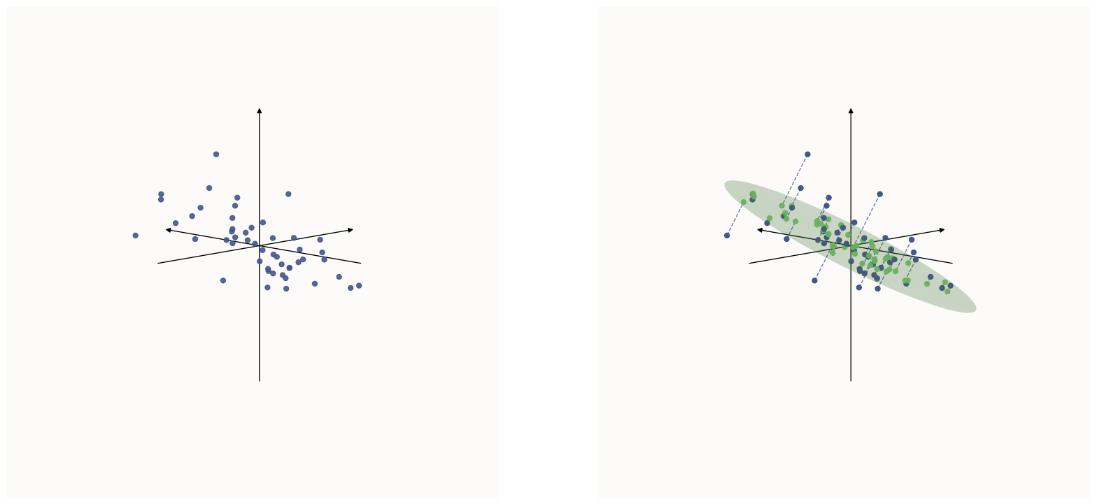
![PCA-like 2D]() How one might represent a 3D dataset in 2D space by projecting it down onto a plane
How one might represent a 3D dataset in 2D space by projecting it down onto a plane $W^\top W x$, aka $W^\top h$, is the decoded vector. The decoding operation (applying $W^\top$) simply takes the compressed 2D representation ($h$) and projects it out to the higher dimensional space (same as the input space). Note that even though $W^\top h$ lives in $\mathbb{R}^n$ (a high dimensional space), its effective dimensionality is that of $h$ (2D), since no matter how you linearly transform (stretch & scale) a 2D set of points, you can never make it more than 2D. Note: In real neural networks, the decoding function is not simply a linear function like $W^\top$, but some more expressive non-linear function. The decoding function represents the construction of output features (or in this case, the reconstruction of input features, because the model is trained to reconstruct its inputs) from a more compressed representation ($h$).
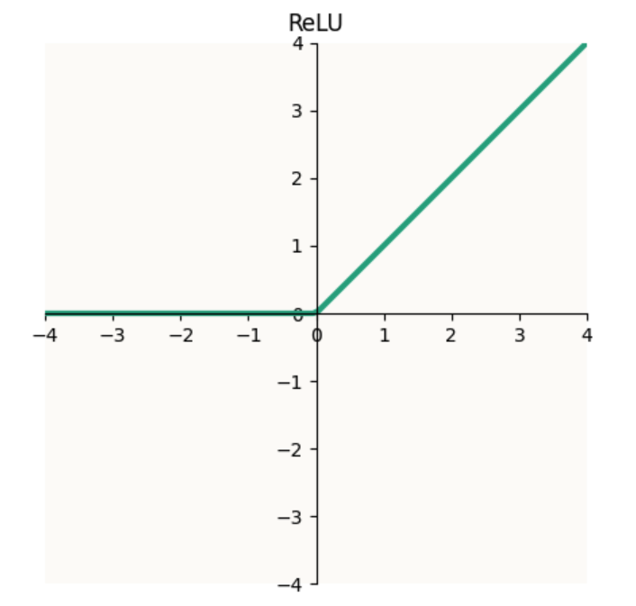
$\text{ReLU}$, the most exciting part, is the non-linear function that is magically able to extract more dimensions of information than exists in the latent space (2). We will see how this works in a while. Mechanically, $\text{ReLU}$ simply takes the max of $0$ and its input value. It’s useful to think of this as clamping values to $> 0$:
![Graph of ReLU]() Graph of the ReLU function
Graph of the ReLU function- $b$, the bias. The bias is, in my opinion, the most deceptively simple part of the linear layer. Intuitively, it’s simple: adding a bias simply shifts everything by an offset. $(W^\top W x + b)$ is basically $W^\top W x$, but $b$ distance away from the origin. But, this bias is incredibly powerful, and without it, the ReLU toy model will be able to encode much fewer features ($2m$, instead of infinite), as we’ll see below.
Why is this toy model worth our time?
It captures basically all of the properties of actual linear layers in deep models. I’ll just list 2 key reasons that this toy model forms a good surrogate for large model components:
- This toy model is basically a “Linear Layer” (although the name has “Linear” in it, in deep-learning parlance, it just means one linear transformation followed by a non-linear activation function like ReLU, hence it’s not linear), which are the basic building blocks of ALL deep models
- This toy model implements compression and decompression, which are key behaviors of ALL deep models
Many of the local behaviors of deep models can basically be studied with this toy model.
ReLU: Free Dimensions, Somewhat
So, in the world of linear transformations, one can never extract more dimensions of information than the minimum that was available at any point. For example, in the above illustration that I’ll paste below, we transformed a 3D dataset into a 2D one. But, given the 2D points (green), you can never reconstruct the original 3D points, because you don’t know how far along the dotted lines they originally were away from the plane.
 How one might represent a 3D dataset in 2D space by projecting it down onto a plane
It follows that when you’ve compressed a $10,000$-dimensional vector to $2$ dimensions, like Anthropic did in the problem set-up, you would not be able to construct the original vector. However, throw in a non-linearity and some sparsity in your data points and you can actually reconstruct the original training data fairly well, sometimes without any training loss! How does this happen? Let’s take a look.
This discussion will pertain solely to the $\text{ReLU}$ non-linearity. The intuition will transfer somewhat to other activation functions, but activation functions have other kinds of inductive biases that will likely cause the representation of features that models end up learning to be different. This is out of the scope of this discussion
We start by considering the dataset - our dataset is perfectly sparse; Anthropic’s dataset was effectively perfectly sparse on average. This means that instead of having vectors that point in random direction in space, you essentially have the standard basis vectors (axial lines):
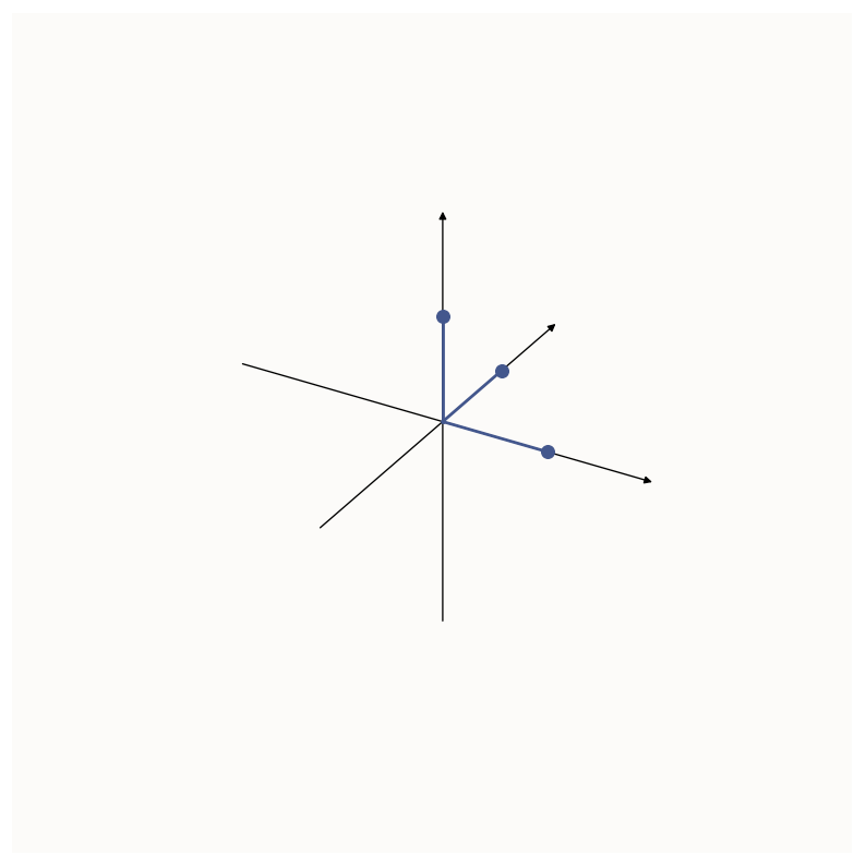 The three standard basis vectors in 3D space
I know that we are operating in high-dimensional input space (e.g. $\mathbb{R}^{10,000}$), but we can only focus on the dimensions where there is data with non-zero entries in that dimension. Suppose we have only 3 data points, then we can basically only look at the 3 dimensions where the data points are non-zero in. Let’s look at how these 3 ‘data archetypes’ can be represented in a 2D latent space. There are 2 explanations:
Explanation 1: The effective dimensionality of the points is low (2D)
In this case, but only in this case, this is correct. You can observe that the 3 data points (the axial vectors) form a plane (a “2D simplex”). Since the effective dimensionality of the data is 2, then of course we can represent it without loss of information in 2D. However, it only works in the case of trying to represent $n$-dimensional data in a $(n-1)$-dimensional latent space. In general, $n$ points in $n$-dimensional space will form an $(n-1)$-dimensional simplex. If your latent space is coincidentally also $(n-1)$-dimensional or bigger, this is fine and dandy, but if your latent space is smaller than $(n-1)$ dimensions, then it will not be able to capture your $(n-1)$-dimensional object perfectly, and this explanation does not suffice.
Explanation 2: “Wrapping” the Latent Space Around The ReLU Orthant
This is not quite the most concise why to explain it yet, but I want to walk through and build up the logic towards the final explanation. A helpful way of thinking about what ReLU does is that it clamps values to be $\geq 0$, i.e. that it snaps all points to the edges of the positive half-space (1D) / quadrant (2D) / octant (3D) / orthant (higher-D), and so on. Let’s see how this clamping visually looks in 1 to 3 dimensions:
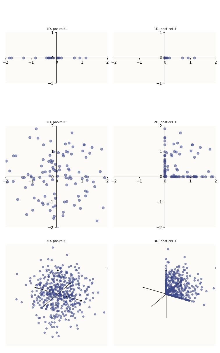 Before (left) and after applying ReLU (right)
Privileged Basis
Notice how, because $\text{ReLU}$ effectively zeros out all negative values, many points are snapped against the positive edges of the positive orthant. This means that a lot of the post-ReLU points are scalar multiples of the axial vectors. Visually, you can see this happening by observing that the axis lines are particularly packed with data points in the right column. This also means that ReLU is particularly good at extracting axial vectors, which is what breaks the rotational invariance (“symmetry”) that is otherwise present in purely linear systems - the axial vectors are hence “privileged,” to borrow the term from Anthropic.
Also, because we are working in the ideal case where the data points are axis-aligned, this is particularly convenient for us, because the type of points that ReLU loves to output (axis-aligned), is exactly the type of points that we are looking to reconstruct. This may look like a beautiful coincidence, and you may think that in real models, you can’t expect axis-aligned vectors or features like this, but the reality is the these things are actually super common! By the end of this section, hopefully the intuition behind how ReLU gives us free dimensions is clear, and it’ll become obvious why learning such axis-aligned feature vectors is beneficial to the model, and is hence what happens in real models.
“Wrapping” a Piece of Paper Around A Table Corner
Because $\text{ReLU}$ sort of “wraps” your data points around the positive orthant at the origin, this mechanism has the effect of giving you “free dimensions,” sort of like how wrapping a piece of paper (2D) around a table corner warps it into a 3D shape, or how wrapping a piece of rope (1D) around the corner of a ruler (2D) makes it 2D. I want to point out that this is not quite a perfect analogy - when you wrap a piece of paper around a table corner, the contact point acts as a pivot, and segments of the paper rotate about the pivot (corner) to meet the surfaces of the table, but ReLU is a little different; instead of rotating regions of the paper about the pivot, it simply projects those regions down onto the surfaces of the table. It’s more of a perpendicular “collapse” onto the surface than a rotation. The dotted arrows in the illustrations below show what this collapse looks like.
Goal: Position the Paper to Wrap a Certain Way
With this paper analogy, notice that the pivot point on paper is quite literally, pivotal, in the sense that different regions of the paper on different sides of the pivot will be collapsed onto different edges / faces of the table. Bringing this back to positive orthant, you can see how the lower-dimensional latent space (2D paper in this case) pivoted about the positive orthant (table edge) at the origin, can be split into 3 regions, each wrapping around the positive orthant in a different way. Now, depending on where you find yourself post-wrap, you could encode any of the 3 features. E.g. if you find yourself along the $x$ axis (edge), you represent an activation in the $x$ feature; if you find yourself along the $xy$ face, you represent activations in the $x$ and $y$ feature. However, note how it is impossible to represent activations in all 3 features (dense) at once because that requires you to be inside the volume of the positive orthant, which is against the rules of the wrapping action ($\text{ReLU}$).
Note how the different “regions” of the paper are basically cones (sectors) of space around the pivot point, like a pie-chart centered at the pivot point. These sectors correspond to areas of the paper that will be wrapped onto the various faces or edges of the positive orthant. The crux of being able to reconstruct each of the original features cleanly is to have sectors that correspond to areas that will wrap onto each of the edges of the cube, because the edge represents an activation of only 1 feature. Again, the goal is to be able to construct these perfectly sparse (1-hot) original inputs. Because this is the goal, we’ll give this criteria a name and a more precise definition:
Unique Single Positive Value (USPV) Criteria
The latent representation of $e_i$ must have a positive $i$-th element and all other elements $\leq 0$.
As we will see, achieving this is not always possible for all values of $n$ and $m$. The constraint here is that you don’t get full freedom to draw your sectors however you want, because the sectors are largely decided by the geometry of the cube, and how you angle the paper about the pivot point. To illustrate this, let’s walk through a lower-dimensional case (feel free to re-read this paragraph, replacing “paper” with “rope” and “cube” with “ruler corner”).
How to Place Rope Properly
In a lower-dimensional version of the wrapping problem, where you wanted ReLU to be able to construct 2 features from a 1-dimensional latent, the analogy is to wrap a piece of rope around the corner of a ruler. You can simply do this:
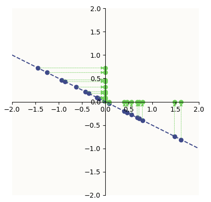 Data latents (purple) being ReLU-ed onto the positive orthant
Notice that the purple dashed line illustrates such a 1D line (rope). The origin (the corner of the ruler) splits the rope into 2 regions - 1 with only positive vertical-axis values and the other with only positive horizontal-axis values - each snapping onto a different edge of the ruler. These correspond to the latent representation of each of the features, and fulfill the USPV Criteria.
If you looked from the under-side of the line (from the bottom-left to the top-right), you would see the axial vectors as the feature vectors (entries of $W$, since $W \in \mathbb{R}^{1 \times 2}$).
How to Place Paper Properly
If you wanted to arrange 3 features on a 2D plane (in a 3D space) to be able to reconstruct the 3 standard basis vectors after ReLU, there is such a similar way of arranging your latent representations, fulfilling the same criteria:
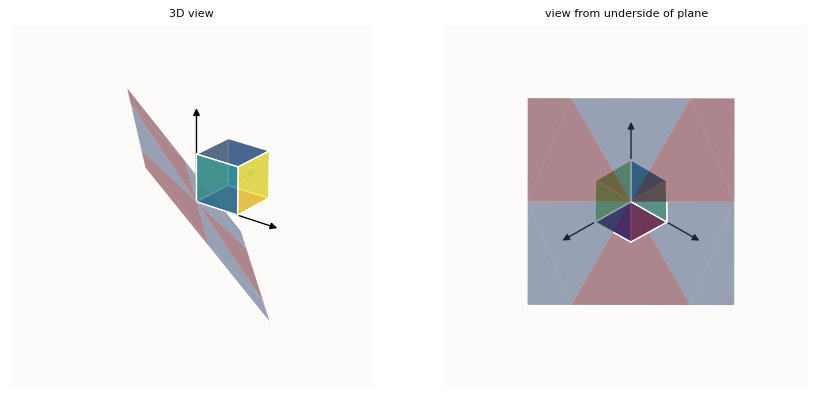 Data latents (on the plane) being ReLU-ed onto the ReLU hypercube in 3D
If you looked from the underside of the paper so that you can see it face-on, you will be able to construct the sectors demarcating the regions that wrap onto different edges / faces of the cube. Note that points in the bluish purple regions of the plane (the latent space) fulfill this criteria and will get snapped onto the edges of positive orthant (axis lines), while points in the red regions of the plane do not, and will get snapped onto the faces of the positive orthant, as opposed to the edges.
If you wanted to compress your original 3D sparse data points onto a 2D plane and be able to reconstruct them this way, then you should ensure that each feature gets projected down (via $W$) into the correct purple cone. This means that the first column of $W$ (a.k.a. $W_1$), which is a 2D vector, has to be in the purple cone that would get snapped to $e_1$ by $\text{ReLU}$, $W_2$ has to be in the other corresponding purple cone, and likewise for $W_3$. This is one such configuration of the columns of $W$, which is illustrated by in Anthropic’s Toy ReLU autoencoder that was trained to reconstruct 3D points with a 2D latent space:
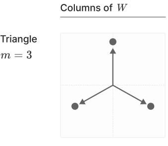 Anthropic’s ReLU autoencoder features (rows of W), image from their paper. Note that m in this image represents n in this post.
Even though we (and Anthropic) achieve the geometrically perfect solution (the 3 vectors are equally spaced apart), in reality, the 3 feature vectors do not have to be equally spaced apart, because they only need to be in their respective purple sectors - there is some wiggleroom. This intuition generalizes for wrapping higher-dimensional hyperplanes around even-higher-dimensional hyperplanes, but is not something we can visualize. Now that we have given up trying to visualize, the question then is - how high-dimensional can a hypercube be for us to be able to be able to wrap an $m$-dimensional hyperplane such that these purple sectors exist? Turns out, the limit is $n = 2m$, for which the purple sectors are literally just lines (cone with no volume) - there’s no wiggleroom! For example, when we try to represent the four $4$-dimensional standard basis vectors on a 2D plane such that $\text{ReLU}$ can snap them back onto their respective edges, the solution for $W$ is just a set of 4 lines (yes, this is what 4D hyper-cube looks like when projected onto a 2D surface):
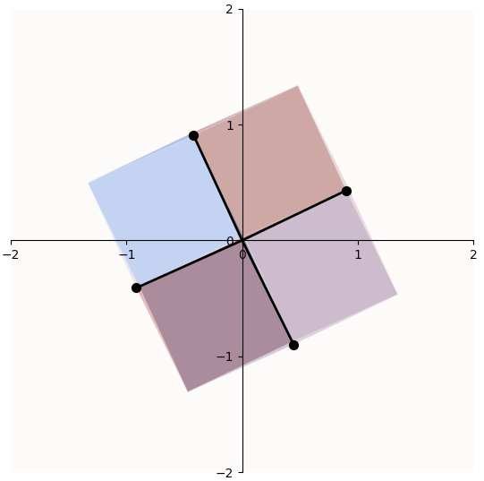 Four 4D axial vectors embedded into 2D space, + some rotation
This is precisely the job of $W$: their columns act as feature vectors, while their rows act as the span of the $m$-dimensional hyperplane in $n$-dimensional space.
Note that this description of $W$ is specific to this context where the compression weights $W$ are the same as the decoding weights ($W^\top$). In reality, they are commonly different, and so you have something like $y = \text{ReLU} (MWx + b)$, hence it would be that the columns of $W$ here that act as feature vectors.
The role of $W$ (Refresher on Basis Transforms)
The model simply wants to train $W$ such that:
- The columns of $W$ (feature representations) have as little interference as possible; orthogonal if possible
- The rows of $W$ define an opportune orientation in $n$-dimensional space such that the feature vectors uphold the Unique Singular Positive Value criteria.
The rest of this section is about the intuition of linear transformations and change of bases; feel free to skip if you have fresh memory of this linear algebra.
If you don’t have a very intuitive understanding of linear transformations, then what I wrote above about the “job of $W$” probably sounds very unobvious, so I’ll quickly illustrate the connection between the plane, the ReLU hypercube, and $W$.
We’ve established that to get the free dimensions via the ReLU Hypercube explanation requires you to rotate your plane (an $m$-dimensional object, in this case, 2) in $n$-dimensional space properly such that when you view the axis lines from the underside of the plane, they fall into their respective sectors of the plane that fulfill the criteria of having 1 positive entry and all else being non-positive. In linear algebra, applying a matrix to a vector (e.g. $Mx$) simply re-interprets $x$ to be not in the standard axes, but in the axes denoted by the columns of $W$. There will be a section on this from my linear algebra primer I’ll release in the future, but for now, here is a quick image of what I mean:
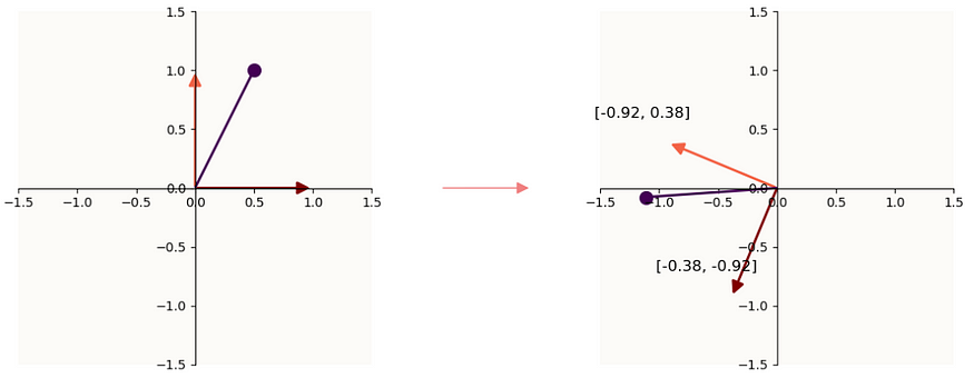 Left: an example vector x (purple). Right: Mx, where the maroon and orange lines are the columns of M
If $M$ were a tall matrix (more rows than columns, i.e. each column is tall), then the changed basis simply just lives in higher-dimensional space. If $M$ were a wide matrix (more columns than rows, i.e. each column is short), then in addition to changing your basis, you’re also reducing the dimensionality of $x$, because $x$ is going from a num_columns-dimensional vector to a $Mx$, a num_rows-dimensional vector.
So if we have $x \rightarrow Wx$, this means that the 2-dimensional columns of $W$ represent the axial vectors of the latent space (a 2D plane) in a 2D world. If we further have $Wx \rightarrow W^\top W x$, this means that the 3-dimensional columns of $W^\top$ represent the axial vectors of the latent space (same 2D plane) in a 3D world. This is why the rows of $W$ act as the span of the $m$-dimensional hyperplane in $n$-dimensional space.
Further, notice that because applying $W$ to $x$ is a reinterpretation of $x$’s entries as values in each of the columns of $W$, this is a remapping of $x$’s features from the standard basis world (e.g. first entry $=$ first feature $= [1,0,0]$), to the $W$ basis world (e.g. first feature is now represented via $W$’s first column - a 2D vector, instead of $[1,0,0]$). This is why the columns of $W$ act as feature vectors.
Now then, it becomes obvious that $W$’s role over training is just to adjust it values properly such that it defines a good $m$-dimensional hyperplane in $n$-dimensional space, such that ReLU can recover all the free dimensions that it needs to perfectly reconstruct the $n$-dimensional vectors with only an $m$-dimensional intermediate representation.
Limit of number of Free Dimensions
I find this intuition very clear: if you pivot a hyperplane about the $n$-dimensional hypercube at the origin and look at the hypercube from the underside of the plane, you can always find a way to rotate the plane about that pivot point (akin to adjusting the rows of $W$) until you can see all the axial vectors (edges of the hypercube). But again, this only works (fulfills USPV criteria) for $n \leq 2m$.
In general, the combined powers of $W$ and $\text{ReLU}$ can only perfectly reconstruct up to $n = 2m$-dimensional axial vectors from an $m$-dimensional latent space. This is because you cannot select a set of $(n > 2m)$ $n$-dimensional vectors, where they satisfy the requirement of 1 positive element in a unique position and all else being non-positive, while having them all be on the same $m$-dimensional object. This means that, for example, a 2-dimensional latent space is expressive enough to reconstruct up to 4 dimensions (if we only care about the axial vectors), a 3-dimensional latent space can reconstruct up to 6 dimensions, and so on. This is great, but it’s definitely not infinite.
Repeat: four 4D axial vectors embedded into 2D space, + some rotation
Proof (thanks David): the upper bound for this (i.e. $n = 2m$) becomes clear when you rephrase the whole USPV criteria charade into: how many vectors can you squeeze into $m$-dimensional space such that no 2 pairs of vectors have a positive ($> 0$) dot product? The solution is just to take all anti-podes of every dimension, so that gives us $2m$.
So, $W$ and $\text{ReLU}$ are definitely not sufficient to account for what Anthropic found - “in fact, the ReLU output model can memorize any number of orthonormal training examples using $T$-gons if given infinite floating-point precision,” where $T$ represents the size of the dataset. The memorized training examples have these latent representations:
 Latent vectors of datasets as T increases (under a certain threshold limit), image from their paper
So how on earth does this happen? This is where the bias $b$ comes in.
The role of $b$
By now, we observe that: trying to represent more than $2m$ axial vectors in an $m$-dimensional latent space will violate the USPV criteria. The intuition for that is basically that in an $m$-dimensional latent space, you can only fit $2m$ orthogonal pairs of antipodal lines. If your vectors are forced to be less than $90^\circ$ apart from each other, then you get some interference.
It’s time to introduce the magic of $b$ that would illustrate why the “Wrapping Paper” analogy is not quite the best way still to think about why $\text{ReLU}$ can hydrate more dimensions that the bottleneck number of dimensions. It turns out, $b$ can basically absorb all that interference by trading off some “sensitivity”. Let’s see how that works. Much of the proof was worked out by Henighan in this Google Colab Notebook.
The intuition thus far was for the latent space (a plane in all our examples so far) to be pivoted at the origin, but it doesn’t have to be pivoted at the origin. In particular, you could add a negative bias in all dimensions such that you can shift the latent representations away from the origin, into the region of space where all dimensions are negative:
 Feature representations in latent space, with bias
This isn’t super useful, because if all your features were represented in the negative regions of space, $\text{ReLU}$ would come along and zero everything; you have no information. However, you can shift the feature wheel in a way such that only feature vector $i$ is positive in dimension $i$, while the rest of the feature vectors are non-positive in dimension $i$:
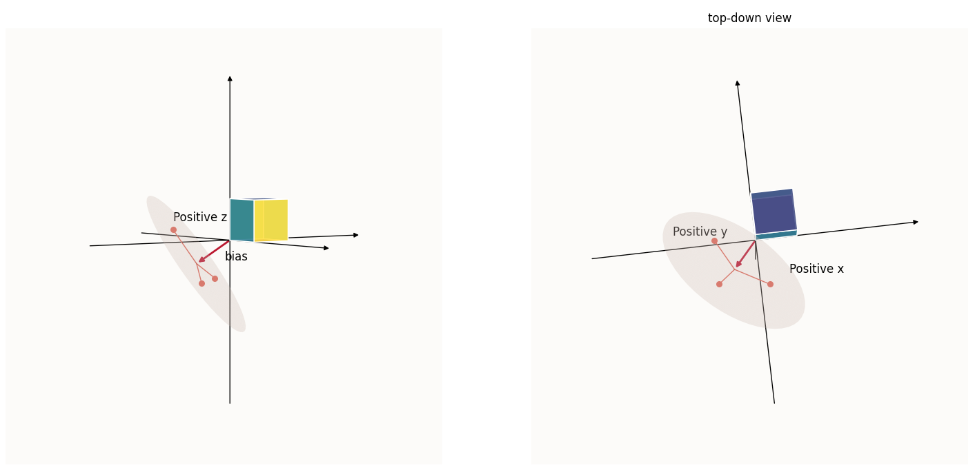
In the left picture above (side-view), notice how only 1 feature is in the positive region along the $z$ (vertical) axis, and when we take a top-down view as in the right picture, only 1 feature is in the positive $y$ (vertical) axis, and likewise for the positive $x$ (horizontal) axis.
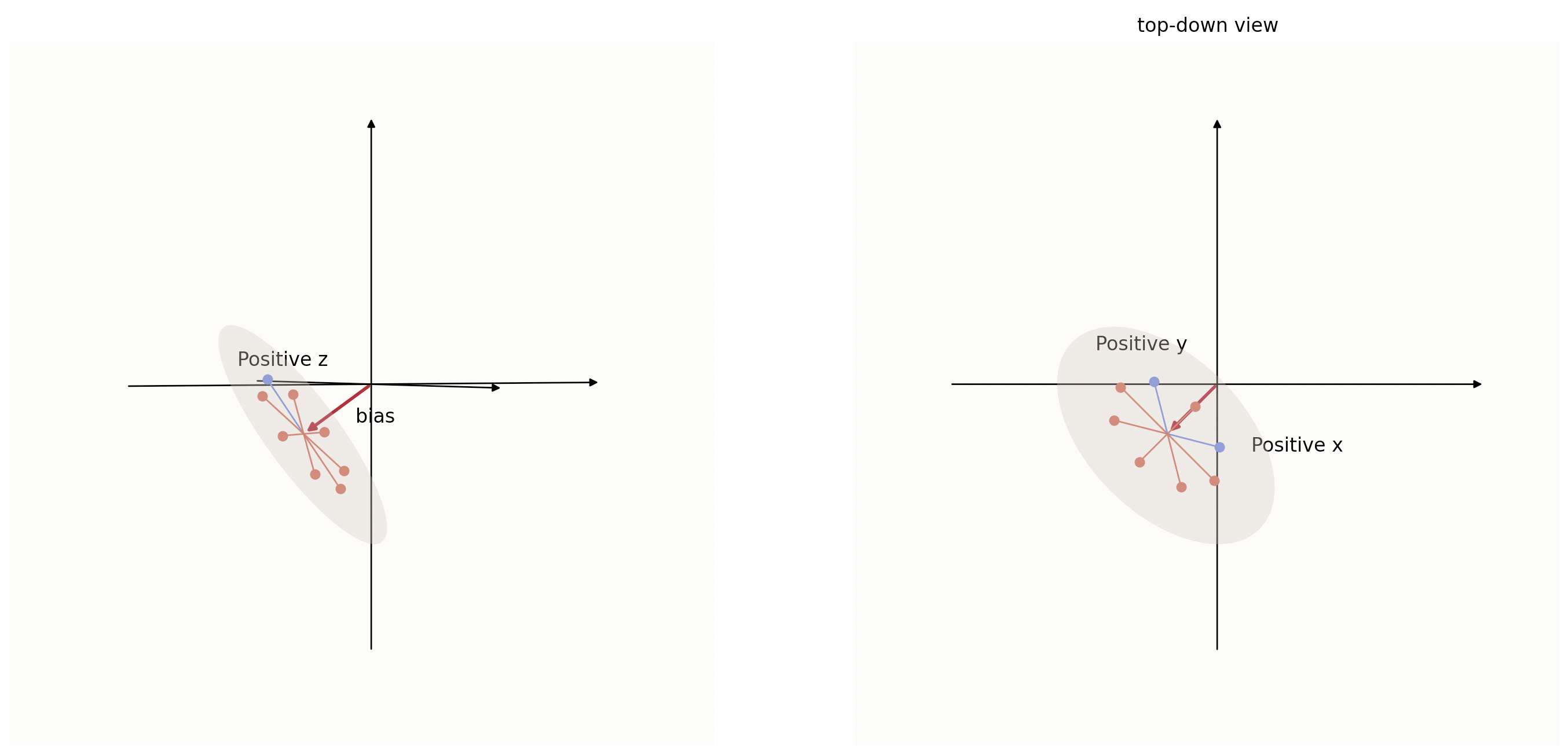
Explanation 3: A Superposition of Half-Spaces
Now we’ve arrived at what I believe to be the most accurate, and intuitive characterization of the latent space: a superposition of half-spaces. You can see that $\text{ReLU}$ splits every dimension into 2 complementary half-spaces, 1 for the positive region (where the feature corresponding to that dimension is “active”), and 1 for the negative region (where the feature is silent). Each $(W_i, b_i)$ pair is responsible for determining how the latent space is split into the half-space pair corresponding to that feature.
The above illustration is of 3 features being embedded in a 2D latent surface in a 3D universe with just 3 vectors. If you recall, we already know that with a 2D latent surface, you can represent up to 4 features while fulfilling the USPV criteria without $b$, but remember that having no bias only works for up to $2m$ vectors. If we have 8 $8$-dimensional axial vectors projected down onto a 2D wheel similarly, then the shifting is necessary to ensure that each one of those USPV criteria-fulfilling regions only has 1 feature vector:
Note: In the above image, with our specific choice of 3 (of the 8 total) dimensions to visualize, we can only see 3 out of 8 feature vectors being in the correct regions that make them fulfill the USPV criteria, but that is merely because we are unable to visualize an 8-dimensional space. If we could plot the above wheel in an 8D space as opposed to a 3D one, we would see that all 8 feature vectors are in their correct respective regions.
Can this really generalize to higher dimensions?
The above claim that a shift ($b$) can really be defined so as to fulfill the USPV criteria for all $n$ dimensions isn’t intuively obvious because we can’t visualize more than 3 dimensions, so we can fall back on analysis to see that this really works. Here is where I will liberally quote the work of Henighan, in that Colab Notebook. This section is more mathematical analysis and less intuition, so feel free to skip it.
Henighan starts of by declaring the dataset $X$ the identity matrix, without loss of generality. This works, because thus far we’ve been assuming that the dataset is just points that align with the axis lines. This means that the data points (the rows of $X$) are one-hot, with their activated element being in unique positions. The identity matrix is just a neat way of arranging these rows, with the $i$-th row being active in the $i$-th position. This makes the objective of the ReLU toy model to reconstruct the identity matrix:
\[\begin{align*} y & = \text{ReLU} \left( X W^\top W + b \right)\\ \Rightarrow I &= \text{ReLU} \left( W^\top W + b \right) \end{align*}\]This means that for this to work, the diagonal entries of $(W^\top W + b)$ need to be the ONLY entries $> 0$; hence the goal becomes to find $W$ and $b$ such that this is true.
He starts off with an a guess for $W$, based on the assumption that the columns (2D vectors) of $W$ will represent vectors that are spaced out evenly over a circle:
\[\begin{align*} W = \begin{bmatrix} \cos(0) & \cos(\phi) & \cdots & \cos(-\phi) \\ \sin(0) & \sin(\phi) & \cdots & \sin(-\phi) \end{bmatrix} \text{, where } \phi = \frac{2 \pi}{\text{num examples / features}} \end{align*}\]Note that we are merely trying to find a $W$ and $b$ such that we can reconstruct the identity matrix; we make no claim on whether it’s guaranteed or even likely for the model to be able to learn (via Gradient Descent) such a $W$ and $b$ from a randomly initialized set of weights.
And so, $W^\top W$ looks like this, after a bunch of massaging with the trigonometric identities:
\[\begin{align*} W^\top W = \begin{bmatrix} \cos(0) & \cos(\phi) & \cos(2\phi) & \cdots & \cos(-\phi) \\ \cos(-\phi) & \cos(0) & \cos(\phi) & \cdots & \cos(-2\phi) \\ \cos(-2\phi) & \cos(-\phi) & \cos(0) & \cdots & \cos(-3\phi) \\ \cos(-3\phi) & \cos(-2\phi) & \cos(-\phi) & \cdots & \cos(-4\phi) \\ \vdots & \vdots & \vdots & \ddots & \vdots \\ \cos(2\phi) & \cos(3\phi) & \cos(4\phi) & \cdots & \cos(\phi) \\ \cos(\phi) & \cos(2\phi) & \cos(3\phi) & \cdots & \cos(0) \\ \end{bmatrix} \end{align*}\]Let’s make it clearer by looking at the matrix in visual form (if you had $10$ 10D vectors now):
 A visual depiction of W.T @ W
I’ve highlighted the maximum value of each row (column too) in the above image. Remember that because $Y = \text{ReLU}(W^\top W X + b)$, and $X = I$, each row here represent the pre-ReLU, pre-bias representations of each data point. From here, it’s obvious that you can just subtract the second-highest value of each row (i.e. $\cos(\phi)$) from every single value, and every row will just have ONE value that is $> 0$ - the blue entries, a.k.a. the diagonal. This explanation works for any $n$, so it will indeed generalize to any $n$.
One small nitpick is that Anthropic wrote that this set up of embedding $n$-dimensional vectors in $m=2$-dimensional latent space can memorize “any number of examples [or features]”, but it’s obvious here that it’s not really any number of features; it’s just any number that is $\leq n$, because once you have $n + 1$, by the pigeonhole argument, there will be at least 1 USPV criteria-fulfilling hyperquadrant with more than 1 example / feature vector in it. That said, if you allowed $n$ to increase with your number of examples / features, then it really is infinite. This is where the added requirement of having infinite floating point precision also makes sense, because as $\phi \rightarrow 0$, the difference between $\cos(0) = 1$ and $\cos(\phi)$ also tends to $0$.
$b$ Trades Off Sensitivity to Absorb Interference
Note that if you try to arrange more than $2m$ vectors on a $m$-dimensional hyperplane, the vectors will necessarily not be orthogonal - there will be some interference. To be able to reconstruct totally sparse (1-hot) features still, you have to absorb the inference somehow, and $b$ does this by shifting the feature wheel into the negative region.
Notice that in the above picture, the length of the part of each vector that is in the positive region in that dimension is shortened. For example, only a very short portion (the tip) of the vector labeled “positive $z$” has a positive $z$-axis value (“activated”). Most of that vector is in the negative region (silenced). Same goes for the “positive x” and “positive y” vectors. This means that for that feature to be reconstructable, the original input’s value in that feature needs to be more than a certain threshold ($b_i$). A small value of the feature ($< b_i$) will not be reconstructable because its representation in the latent space is $< 0$ in dimension $i$. I find this intuitive - the bias is commonly explained as a threshold that a neuron needs to be activated beyond in order to make the neuron “fire”. If it’s too weak, the neuron simply won’t fire.
An Actual Picture of Latent Spaces
So we’ve shown how $W$, $b$, and $\text{ReLU}$ work together to be able to superpose an infinite number of vectors into a lower dimensional latent space while side-stepping the problem of interference. We can now attempt to illustrate what the latent space of our ReLU toy model looks like, which will really solidify a geometric understanding of latent spaces.
For a simple case of an ideal autoencoder (ideal meaning that the autoencoder learnt a symmetric configuration of features representing ALL features) compressing $n = 6$ basis vectors into a $m = 2$-dimensional latent space, here is a plot of what I call the “latent zones” of the 6 features.
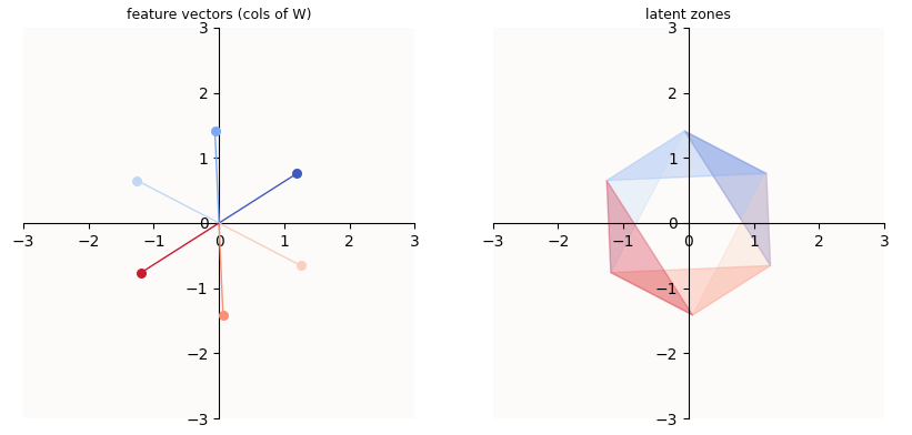
On the left, you can see the column vectors of $W$ arranged into a perfect circle. On the right, I plotted the regions of the latent space (2-dimensional) that correspond to an activation of the $i$-th feature. For example, in order to activate (reconstruct) the orange feature in the reconstructed vector, the hidden vector computed by the model needs to be in the orange region.
Plotting quirks: Notice that the latent space seems to be limited to a hexagon, rather than the entire 2D subspace. This is merely a quirk of my plotting logic; since the non-zero entries of our input vectors (the standard basis vectors) are all $1$’s, it is sufficient to plot a portion of the latent space that contains all the columns of $W$ in 2D (equivalent: all the columns of $WI$ in $n$-dimensional latent space). Such a portion of space is simply given by the outline drawn by enumerating the columns of $W$ in a clockwise fashion.
To fully appreciate why the activation zones are as such, I illustrate the latent space (a planar hexagon) in a 3D space:
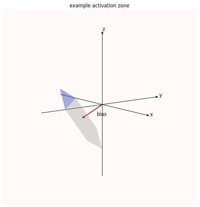
I’ve also highlighted the activation zone of the $z$-th feature, which is simply the part of the latent space with $z > 0$. It is now also obvious that the $z$-th value of the bias is the lever which controls where that blue sliver starts. A $b_z$ that is more negative means that the latent hexagon is pushed down further along the $z$-axis, meaning that the sliver of the hexagon that satisfies $z > 0$ starts further up the hexagon. Conversely, a less negative $b_z$ means that the hexagon will be situated further up the $z$-axis, meaning that the sliver of the hexagon that satisfies $z > 0$ will start nearer the bottom of the hexagon.
I’d also like to point out that the amount of reconstruction a feature gets is hence determined by how much the feature vector extends into its corresponding latent zone:
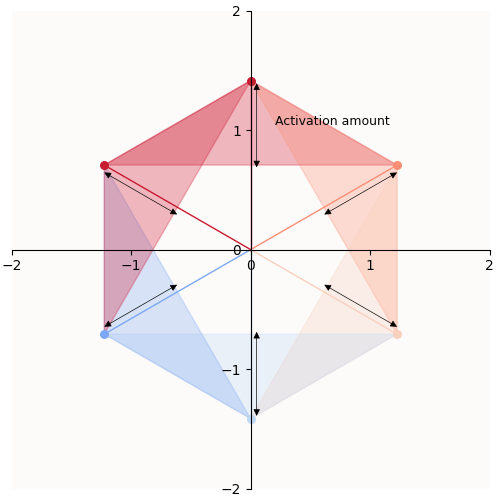 Amount of activation must be equivalent to reconstruction of the feature
The Punchlines
I think the above latent zone plots illustrate crystal clearly what the 2D latent space looks like for our ReLU toy model. Although we only plot 3 out of the 6 dimensions (because we humans can’t visualize more than 3 dimensions), you can already see how $W$, $b$, and $\text{ReLU}$ interact to silence most of the latent space (where the value in the $i$-th dimension is $< 0$, and is hence zero-ed out by $\text{ReLU}$). Notice:
- Interference is completely side-stepped: the latent space is cleverly positioned (pushed in the negative direction by the bias) such that other features are silenced when necessary (e.g. the light blue feature is silent with respect to the latent zones of the blue and light orange feature).
- Reconstruction of features are linear in their latent zones: The more a data-point’s representation lies in a feature’s direction, the more their activation (reconstruction). So long as the magnitude of an input feature overcomes the bias, its reconstruction is linear! This is a very strong direct explanation for why features are generally linear in ReLU models.
- In fact, this illustrates very clearly a fact that sits in broad daylight: neural networks that have only ReLU activations as their non-linearity are piece-wise linear, and their latent zones are superpositions of pairs of complementary half-spaces!
Not So Useful, but also Incredibly Useful
In general, this visualization or mental conceptualization of latent spaces as a superposition of half-spaces (or being piece-wise linear) is not a total game-changer for how we design or optimize neural networks because most (1) deep models have some kind of layer or batch normalization, which is non-linear (I think this doesn’t change the geometry too much though, and ongoing research shows that schemes to “fold away” layer normalization don’t change model expressivity), and (2) well, what are you going to do with that knowledge anyway? Do convex optimization over $2^n$ linear zones of model latents to find the global optimum? 😂
Still, I find this to be an incredibly powerful way to understand latent spaces and the types of compositions of features that are possible. Here are 3 really compelling examples.
- This visualization makes it clear that not only 1-hot features are encodable, but also specific combinations of 2 features!
- It also begins to explain why Anthropic observed that “models prefer to arrange correlated features side by side if they can’t be orthogonal”: because if 2 features are known to co-activate, having them side-by-side creates a region where their latent zones overlap!
- It also begins to explain why Anthropic observed that “models prefer to represent correlated features in orthogonal dimensions” (if they can): because if 2 features are known to co-activate and aren’t side-by-side, then it becomes hard (or impossible) to put those 2 features in the same tegum factor (hexagon in this case) such that you can activate them without activating some 3rd feature. The only way is to have the 2 features be in 2 different tegum factors (orthogonal).
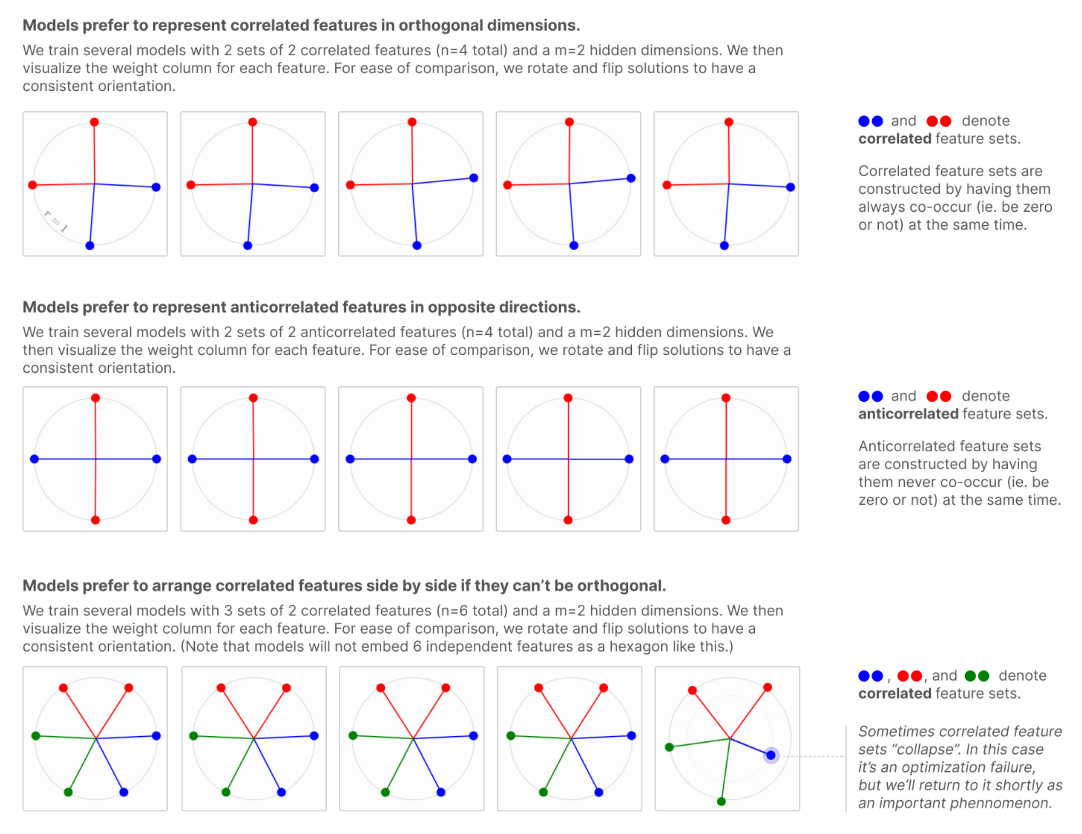 From - you guessed it - Toy Models of Superpositions, Anthropic
Closing Words
The biggest takeaway I hope you have from this post is the mental image of the model latent zones. This has been a really powerful geometric visualization of latent spaces that I’ve found to be absolutely necessary in exploring “Optimization Failure,” my next post. Even if you don’t intend on reading the next post, I think this mental image demystifies what model latents look like, and will be very helpful in understanding a lot of mech interp work that deals with feature representations.