Early this year, Jacob Hilton from Alignment Research Center (ARC) posted about the problem that his team had been tackling, primarily around really mechanistically understanding small (< 1,500 parameters) models. He released his team’s Algo Zoo, with model families of small models of various sizes, with the TLDR being:

They were able to mechanistically describe the smallest 2 models (10 and 32 parameters) but struggled with 432 and more parameters
The generalized difficulty of mechanistically describing models is coming up with a procedure that is at least as efficient as sampling

I really like the focus that is placed on really understanding small models, and find this problem rather interesting in general, so this post will be about walking through some of the post’s findings, deriving and exploring mechanistic descriptions of the small models, and if scope permits, postulating how one might find an efficient way to arrive at a mechanistic description at least as quickly as sampling, or if the comparing the 2 techniques is fundamentally wrong due to the different limitations of each approach (they tell you different kinds of information, after all).

What Counts as a Mechanistic Description?

Hilton’s post expatiates their inability to fully define what a “Mechanistic Description” entails. I will not strive for a formal definition either, but here are some examples of what counts; they all revolve around the idea of “the ability to control”:

You can outline conceptually what the various mechanisms of the model are and hand-define weights to construct the “ideal” mechanisms to achieve no loss.
You can describe precisely what classes of inputs the model will fail on (e.g. “input coordinates falling in this convex cone will produce the wrong answer”).
You can predict what the model’s loss will be given some test dataset sampled from a known distribution.

To me, mechanistic interpretability is all about being able to say with certainty what your model does (i.e. what it can and cannot do), because it is fundamentally a control problem - you understand the model so that you can control and improve it. But as we’ll see, “certainty” is frequently a qualifier that has to be relaxed, due to computational demands.

Problem 1: 2nd Argmax

One of the model families Hilton’s team wrote about was 1-layer RNNs trained to correctly identify the 2nd-argmax of a series of real numbers.

Architecture

All matrix math here is written in math convention instead of torch convention

“The Model $M_{d,n}$ is a 1-layer ReLU RNN with $d$ hidden neurons that takes in a sequence of $n$ real numbers and produces a vector of logit probabilities of length $n$. It has three parameter matrices:”

the input-to-hidden matrix $W^{hi} \in \mathbb{R}^{d \times 1}$
the hidden-to-hidden matrix $W^{hh} \in \mathbb{R}^{d \times d}$
the hidden-to-output matrix $W^{oh} \in \mathbb{R}^{n \times d}$

Hidden Size 2, Sequence Length 2

$M_{2,2}$ is the smallest model (and Sequence Length 2 is a special case since it’s “2nd Argmax” here is essentially “Argmin”), and the team has achieved full understanding of it. The post’s mechanistic description of $M_{2,2}$ offers almost no details, but they do say that an ideal, hand-constructed model, achieves 100% accuracy using these weights:

\[\begin{align*} W^{hi} = \begin{bmatrix} +1 \\ -1 \end{bmatrix}, \space W^{hh} = \begin{bmatrix} -1 & +1 \\ +1 & -1 \end{bmatrix}, \space W^{oh} = \begin{bmatrix} +1 & -1 \\ -1 & +1 \end{bmatrix} \end{align*}\]

This is enough information for me to extract my own mechanistic description of the model.

Mechanistic Description: “Forward Pass / Anthropomorphic”

This section will detail a type of Mechanistic Description that I call “Forward Pass / Anthropomorphic,” because it involves stepping forward through the model, and ascribing a fitting human description to what we think each component (linear transform, ReLU, etc.) is doing.

For the sake of simplicity, I will normalize all weight columns so they have unit length. This will allow me to simply say things like “projection” and “change of basis” without caring about the scaling factor.

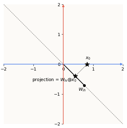
\[\begin{align*} W^{hi} = \frac{1}{\sqrt{2}} \begin{bmatrix} +1 \\ -1 \end{bmatrix}, \space W^{hh} = \frac{1}{\sqrt{2}} \begin{bmatrix} -1 & +1 \\ +1 & -1 \end{bmatrix}, \space W^{oh} = \frac{1}{\sqrt{2}} \begin{bmatrix} +1 & -1 \\ -1 & +1 \end{bmatrix} \end{align*}\]

Step 1: input $x_0$ is embedded (projected) onto the span of $W_{hi}$:

Step 2: ReLU

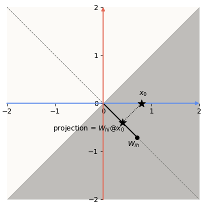
Because a ReLU follows immediately after, the vector space is segmented into a red half-space (first element is preserved through ReLU), and a blue half-space (second element is preserved through ReLU). There’s a cone where the 2 half-spaces overlap, as well as a cone outside either half-space. We can see that positive values of $x_0$ will embed into the blue cone, while negative values of $x_0$ will embed into the red cone. Crucially, this means that all possible values of $x_0$ are preserved.

Step 3: $W_{hh} ( \cdot )$

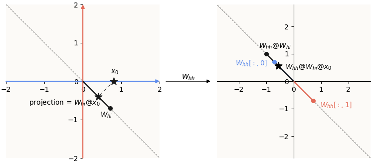
Next, we have to apply $W_{hh}$ to our current hidden state. This means calculating $W_{hh} W_{hi} x_0$. Visually, it’s just a change of basis, where the new basis vectors are simply the columns of $W_{hh}$ (highlighted blue and red); they take the role of the horizontal and vertical axes of the pre-change-of-basis space.

So this is the transformation (pre and post) of the basis via $W_{hh}$:

Step 4: input $x_1$ is embedded (projected) onto the span of $W_{hi}$ (this time I highlighted it orange to indicate that it’s specific to $x_1$):

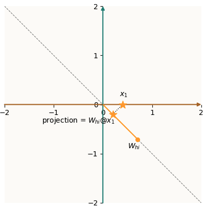
Step 5: Add the current embeddings of $x_0$ and $x_1$ to get sum, followed by a ReLU:

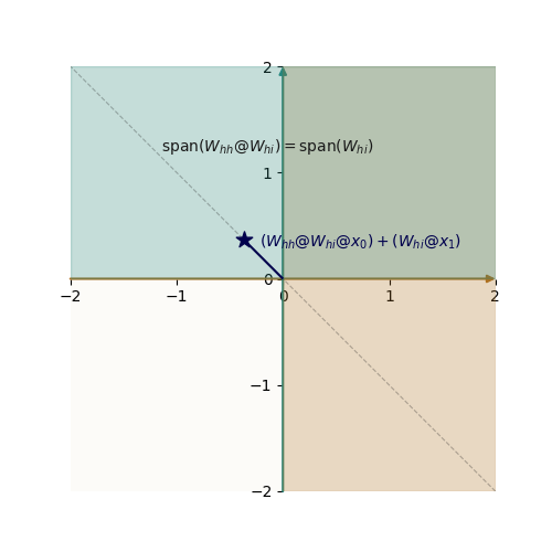
Crucially, we see that:

Positive values of sum get embedded into the blue-green region
Negative values of sum get embedded into the brown region
No values of sum get embedded into the region of overlap; this the region of interference (in this particular case it’s ok, but in general interference is bad - out of scope of this post)
All possible values of sum are represented.

The partitioning of negative and positive sum values into different regions is really convenient for the problem. In this case, having a non-zero $h_2$ corresponds to $x_0 > x_1$ and having a non-zero $h_2$ corresponds to $x_1 > x_0$.

Step 6: $W_{ho}(\cdot)$

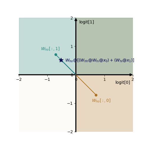
You’ll see that in this case, $W_{ho}$ doesn’t really do much. The partitioning remains unchanged, which is a good thing. This means that logit[0] will be non-zero iff $x_0 > x_1$ and logit[1] will be non-zero iff $x_1 > x_0$.

There are many solutions for $W_{ho}$ that would have preserved this property all the same, including the identity matrix.

Mechanistic Description: “Reverse Engineering / Brute-Force”

There is another way of obtaining a mechanistic description, which I call “Reverse Engineering / Brute-Force.” This entails answering the question: where can my inputs be in order to activate (i.e. achieve non-zero) each output logit? We do this by defining constraints in the output logit space, and tracing back the pre-image to the output constraints, layer by layer. In the end, what we end up with is a set of constraints that describe where in the initial $x_0, x_1$ space your inputs have to be to have a non-0 logit[0], and same for logit[1]. I call these “input zones”:

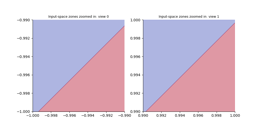
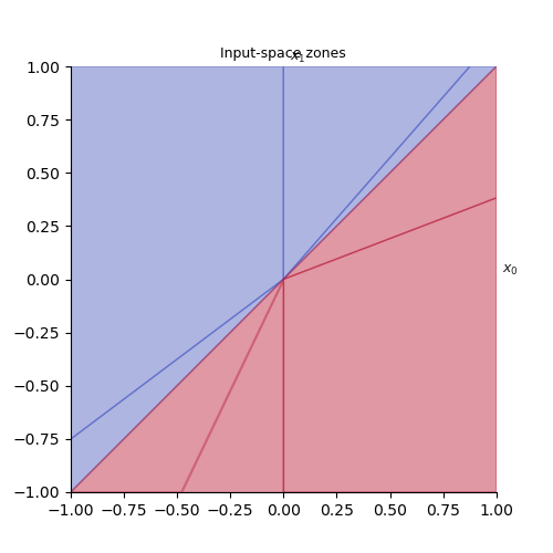Input zones for actual $M_{2, 2}$ (not hand-picked). Blue: model thinks 2nd-argmax is 0, Red: model thinks 2nd-argmax is 1

These constraints are very powerful, because they tell us complete information about what inputs will yield a correct, or incorrect result. We know that the ground-truth for such a plot is simply:

The 2nd-argmax is 0 (i.e. logits[0] > 0) if $x_1 > x_0$ (triangle on the upper side of diagonal line $x_1 = x_0$)
The 2nd-argmax is 1 (i.e. logits[1] > 0) if $x_0 > x_1$ (triangle on the lower side of diagonal line $x_1 = x_0$)

So an example question we can ask is: what volume / area of the groundtruth $x_1 > x_0$ triangle is missing from the blue triangle? What volume of the groundtruth $x_0 > x_1$ triangle is missing from the red triangle? Together, what’s the volume of error? We can get quite specific and exact with the errors:

blue missing volume	`1.2803098280059666e-10 / 2.0`
red missing volume	`0.00048685437030388516 / 2.0`
Fluke volume (i.e. 0-logits classified as blue by default)	`1.2803098280059666e-10`
Total error volume = sum(missing) - fluke	`0.00048685437030388516 / 4.0`
Analytical accuracy within `Uniform(-1.0, 1.0)`	`0.999878286407424`
Empirical sampling (`n=4_000_000`) accuracy	`0.99989122`

Majority of the error comes from red missing volume (i.e. groundtruth $x_0 > x_1$ points being misclassified as blue), which you can see visually when you zoom in to the input zone plots and notice that the decision boundary isn’t exactly on $x_1 = x_0$.

Hidden Size 4, Sequence Length 3

So we explored the Anthropmorphic and Brute-Force approaches for $M_{2, 2}$. The former essentially amounts to Guess-And-Check, where we looked at the weights and intuited what a plausible mechanism is, and checked back to see if the weights actually explain the mechanism. The latter is just clever algebra-bashing. The north-star here is to not use brute-force but also device a mechanism that allows us to avoid Guess-And-Checking, but this is a generally extremely hard problem in mech interp. All mech interp techniques now rely on intuiting / proposing some plausible mechanism, and searching to see if the mechanism exists. In attempting to work our way to a mechanical technique, we need more insight.

Brute-Force

There are a few techniques we may use to interpret $M_{4, 3}$. Just to get things out of the way, I want to say that brute-forcing is possible, since this model is really small. This is something ARC considered “not adequate” - not that they did it (they explored using mathematical arguments instead, but even the approaches they wrote up turned out to be very incomplete and clunky). Following the above technique we used to brute-force our way to a mechanistic description of $M_{2, 2}$, we similarly have input zones for $(x_0, x_1, x_2)$:

Blue: model thinks 2nd-argmax is 0, Grey: model thinks 2nd-argmax is 1, Red: model thinks 2nd-argmax is 2

matplotlib’s plotting / lack of 3D buffering leaves quite a bit to desire. To read more about the technique I devised to perform this (on both $M_{2, 2}$ and $M_{4, 3}$), you can read “Multi-Layer Latent Space Visualization”.

Anthropomorphic

While brute-force was OK in this case (only took ~3 seconds to compute the pre-images), doing so is exponential ($O(2^{\text{hidden dim} \times \text{seq len}})$). This would amount to like $10^{41}$ seconds for $M_{16, 10}$. So, we need to explore possible methods and more mathematical methods that may allow us to search for this mechanistic description more quickly. Algebra-bashing is still very useful because it’s pretty much our only tool for an analytical and accurate computation of a pre-image, but doing this on the entire model is infeasile; rather, it is something we probably have to combine with further mathematical tricks.

To uncover what mathematical tricks we may add to our tool box, we will continue with the anthropomorphic approach to $M_{4, 3}$. Unlike the hand-picked ideal $M_{2, 2}$, this model adds more complexity to our analysis because it doesn’t achieve 100% accuracy. The explanations for the mechanisms are not clean because they obviously don’t work all the time.

Hilton’s team reports that $M_{4, 3}$ achieves an accuracy of 98.5% on a Gaussian input. I instead evaluate its accuracy for 40,000 inputs uniformly sampled between $(-20, -20, -20)$ and $(20, 20, 20)$. I got these accuracies:

Accuracy by ground-truth answer

Ground-truth Answer (idx)	Accuracy
`0`	0.9865 (`n`=13349)
`1`	0.9776 (`n`=13230)
`2`	0.9689 (`n`=13421)

Accuracy by input ordering

Input Ordering (idxs)	Accuracy
`0 > 1 > 2`	0.9767 (`n`=6574)
`0 > 2 > 1`	0.9710 (`n`=6690)
`1 > 0 > 2`	0.9881 (`n`=6611)
`1 > 2 > 0`	0.9667 (`n`=6731)
`2 > 0 > 1`	0.9850 (`n`=6738)
`2 > 1 > 0`	0.9785 (`n`=6656)

There didn’t seem to be a major class imbalance, which would have suggested that the model just de-prioritized learning a certain input ordering or ground-truth answer, so I decided to simply visualize the logits of all the inputs, color-coded by ground-truth class. I also highlighted the constraint cones in this logit-space: one each for:

$x_0 > \max(x_1, x_2)$
$x_1 > \max(x_0, x_2)$
$x_2 > \max(x_0, x_1)$

We can see here that most of the points are correctly classified, with what seems to be 3 major decision groups:

0 > 2 > 1 (orange) and 1 > 2 > 0 (red)
0 > 1 > 2 (blue) and 2 > 1 > 0 (brown)
2 > 0 > 1 (purple) and 1 > 0 > 2 (green)

Notice that each major group contains 2 classes. Some observations:

The 2 classes within each major group share the same answer to the 2nd-argmax question, hence they’re in the same constraint cone
But not only are they in the same constraint cone, they seem to share the same region (coplanar; superposed on top of each other), suggesting shared computational circuitry (symmetry)

Weights

Let’s take a look at $W_{hi}$:

\[\begin{align*} W_{hi} = \begin{bmatrix} 3.9653 \\ 4.6995 \\ -4.7163 \\ -3.9652 \end{bmatrix} \end{align*}\]

Notice that this is just a line:

whose direction is positive in dimensions 0 and 1, and negative in dimensions 2 and 3
whose dimensions (0, 1) seem to be a mirror image of dimensions (3, 2).

If we plot the embeddings $W_{hi} x_0$ in these pairs of dimensions and apply ReLU, we get:

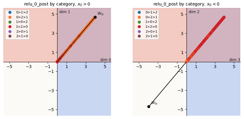
Note that dims (0, 1) preserve positive $x_0$ values (mostly orange since these correspond to data samples where $x_0$ was the largest, which is most likely when $x_0$ is positive), while dims (3, 2) preserve negative $x_0$ values (mostly red points for opposite reason).

Next, let’s take a look at $W_{hh}$:

\[\begin{align*} W_{hh} = \begin{bmatrix} 1.3387 & -2.1996 & 2.6352 & -1.8948 \\ 1.9277 & -2.4339 & 2.7868 & -2.3826 \\ -2.3877 & 2.8057 & -2.4339 & 1.9331 \\ -1.8931 & 2.6429 & -2.1912 & 1.3409 \end{bmatrix} \end{align*}\]

Things to note - more symmetry:

Columns (0, 1) seem to be a flip (permutation) of columns (3, 2)
Rows (0, 1) seem to be a flip (permutation) of rows (3, 2)

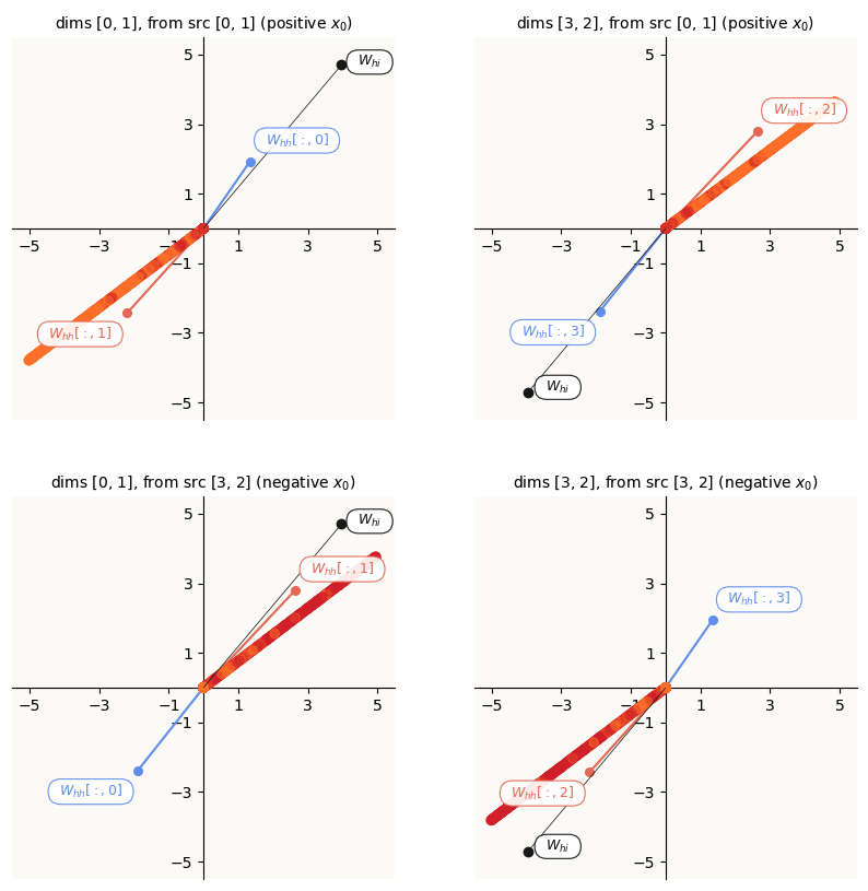
If we think of $W_{hh}$ as a change of basis (COB) just like we did in the case of $M_{2, 2}$, we can visualize the COB by looking at how the axis lines are mapped onto the columns of $W_{hh}$. There’s just one complication - because we’re in 4D now, and we can only really visualize a COB in 2 dimensions, we need to pick 2 source dimensions and 2 target dimensions to visualize. Because the natural pairings of dimensions have been (0, 1) and (3, 2) so far, we can visualize the COBs for each combination of these pairs as source and target:

Note (more symmetry):

The top left COB (src [0, 1] -> tgt [0, 1]) and bottom right COB (src [3, 2] -> tgt [3, 2]) are basically doing the same thing.
The other 2 COBs are also basically doing the same thing.

Let’s add in the embeddings $W_{hi} x_0$ to these COB visualizations:

Notice that the source dimensions (0, 1) contain positive $x_0$, while the source dimensions (3, 2) contain negaitve $x_0$.

Now, let’s add in the embedding of the next number in each input, $W_{hh} x_1$. We get some very nice structure for the sum embeddings (just before the second ReLU):

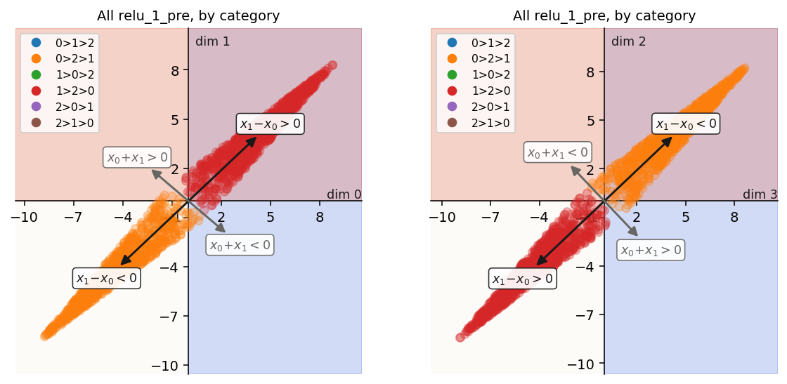
Notice that in each pair of dims, the dark diagonal line (~ first principle component) acts as a “$x_1 - x_0$” feature, which is completely analogous to the $M_{2, 2}$ case. What is basically getting computed is:

\[\begin{align*} \texttt{relu_1_post}_{(0, 1)} &= \begin{cases} W^{hh}_{(0, 1), (0, 1)} W^{hi}_{(0, 1)} x_0 + W^{hi}_{(0, 1)} x_1 & \approx \text{flip} \left( W^{hi}_{(0, 1)} x_0 \right) + W^{hi}_{(0, 1)} x_1 \\ W^{hh}_{(0, 1), (3, 2)} W^{hi}_{(3, 2)} x_0 + W^{hi}_{(0, 1)} x_1 & \approx W^{hh}_{(0, 1), (3, 2)} \text{flip} (x_0) + W^{hi}_{(0, 1)} x_1 \\ \end{cases} \text{ } \, \\ \texttt{relu_1_post}_{(3, 2)} &= \begin{cases} W^{hh}_{(3, 2), (0, 1)} W^{hi}_{(0, 1)} x_0 + W^{hi}_{(3, 2)} x_1 & \approx W^{hh}_{(0, 1), (3, 2)} \text{flip} (x_0) + W^{hi}_{(3, 2)} x_1 \\ W^{hh}_{(3, 2), (3, 2)} W^{hi}_{(3, 2)} x_0 + W^{hi}_{(3, 2)} x_1 & \approx \text{flip} \left( W^{hi}_{(3, 2)} x_0 \right) + W^{hi}_{(3, 2)} x_1 \\ \end{cases} \end{align*}\]

By $\text{flip}$, I mean along the $\begin{bmatrix} 1 \\ 1 \end{bmatrix}$ direction. In all cases, $x_1$ is added to something like $\text{flip}(x_0)$. This encoding of $x_1 - x_0$ is completely analogous to $M_{2, 2}$. However, this time, each $2 \times 2$ block of $W_{hh}$ is rank-2, in contrast to the rank-1 $W_{hh}$ matrix in $M_{2, 2}$. This is why the relu_1_pre scatters span non-zero area now.

This 2 dimensionality is needed, and it turns out that because the $\text{flip}$ operation isn’t an exact mirroring flip (there’s some residual), this residual axis is actually able to encode $x_1 + x_0$. Because we later on need to know where $x_2$ falls relative to $x_0$ and $x_1$, we need to keep both pieces of information about $x_0$ and $x_1$; this residual axis, and hence 2-dimensionality, is needed.

From now on it is useful to treat these embeddings as features for $x_1 - x_0$ and $x_0 + x_1$, which I’ll call $\Delta(x_1, x_0)$.

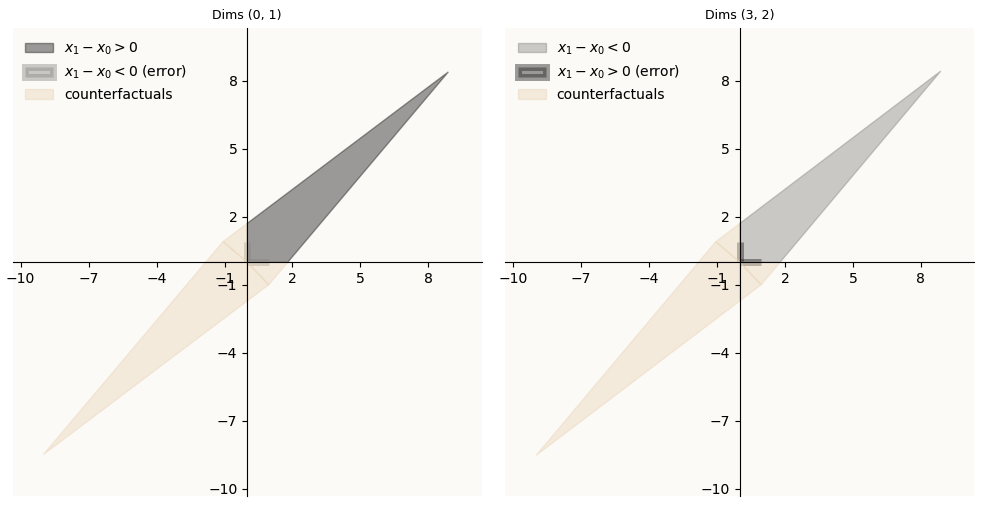
Notice that post-ReLU, we largely “keep” (by this I mean that their embeddings are not the $0$ vector) only points where $x_1 > x_0$ and $x_0 < x_1$ respectively, but not very cleanly. Notice that there are some outliers along the axis lines, not just at the origin.

Let’s transform by $W_{hh}$ again (with several axes overlayed):

Next, I want to inspect how these $W_{hh} \Delta(x_1, x_0)$ triangles get transformed to relu_2_pre. I’ve plotted the pre-addition embeddings ($W_{hh} \Delta(x_1, x_0)$) and post-addition embeddings ($W_{hh} \Delta(x_1, x_0) +W{_hi} x_2$) for $W^{hh}_{(0, 1), (0, 1)} \Delta(x_1, x_0)$:

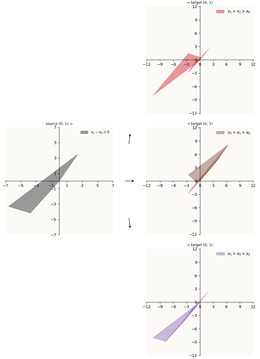
I’ve separated each class’ activation region into distinct plots to make it clearer, but in reality, they all share the same subspace, but there’s very distinct linear separation between the classes, just based on the difference between how $x_2$ relates to $x_0$ and $x_1$ for the classes. When we plot them in the same space, the look like:

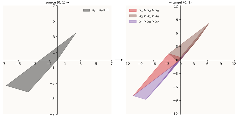
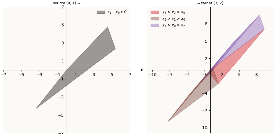
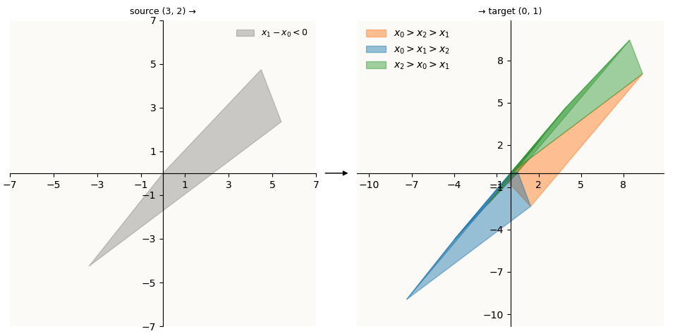
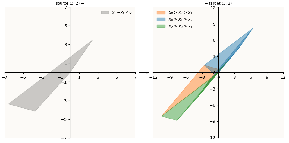
Note that each of these relu_2_pre polygons are not just 1 simple convex hull even though each $W_{hh} \Delta(x_1, x_0)$ was a simple convex hull because I also had to track the “counterfactual regions”, which are the parts of relu_1_pre that had been collapsed to a point or a line (in relu_1_post and $W_{hh} \Delta(x_1, x_0)$) by ReLU. These contribute more convex hulls to the total activation region of where a certain data sample belonging to a given label could be embedded in relu_2_pre space.

If we plot all of these by dimension pairs in relu_2_pre space, we get:

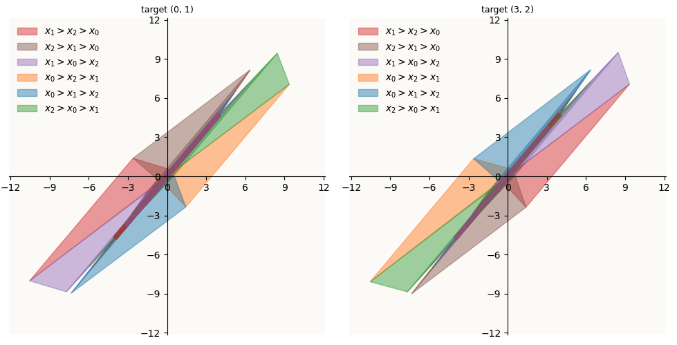
And we can easily see that though there is generally good linear separation, there are regions of overlap, and these regions correspond to prediction errors. I won’t go through the mathematical verification that this is indeed true, but making a scatter plot of the correctly predicted samples and false negatives (color-coded by ground truth) will show you that this is basically true:

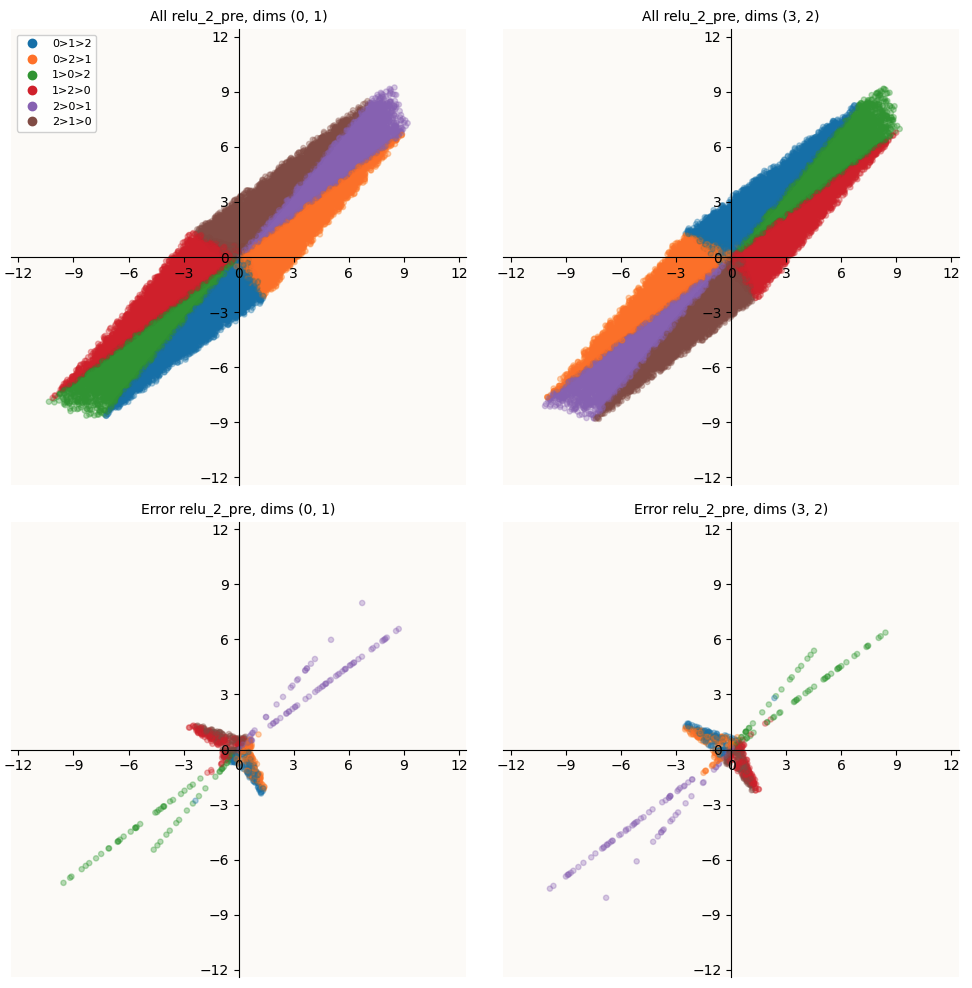
More importantly, this also shows us that by now, we have already obtained a mechanistic description of the model. These convex hulls have known boundaries and calculable distributions, so you have complete information of what the model’s performance is going to be, and whether a given point will be correctly predicted or not.

It all magically works out for us, but how? There is a perfect storm of properties that the model has managed to learn, that achieves this eventual linear separation.

Needed Properties

Here, I will list out the properties needed thus far to make all the components do what they’re supposed to do. Because

1. Symmetry

The fact that $W^{hi}_{(0, 1)}$ and $W^{hi}_{(3, 2)}$ are mirror images (negative and $\approx$ same vector flipped) of each other (and so are $W^{hh}_{(0, 1)}$ and $W^{hh}_{(3, 2)}$) is NECESSARY.

The first reason is because $W_{hi} x_0$ is immediately subjected to a ReLU, which means that in all dimensions, only half of the $x_0$ number line is preserved. In the case of dimensions (0, 1), the positive half is preserved. However, for the model to be able to encode $x_1 - x_0$ completely later on (in relu_1_pre), it needs to be able to receive all possible values of $x_0$. This means $W_{hi}$ MUST have BOTH positive and negative values. This explains the existence of both positive and negative values in $W_{hh}$, but not yet the mirror part.

The second reason is that because the positive-$x_0$ circuitry eventually embeds the $\Delta(x_1, x_0)$ feature in the same relu_1_pre dimensions as the negative-$x_0$ circtuiry, so they MUST share the same representational structure. As a reminder, here’s the rough circuitry again, and observe that both $(+)$ and $(-)$ values of $x_0$ feature in both dimension pairs of relu_1_pre.

$\begin{align*} (+) x_0 \rightarrow \text{ dim }\texttt{(0, 1)} \text{ of } \texttt{relu_0_post} \rightarrow \begin{cases} (-)\text{ orthant of dims } \texttt{(0, 1)} \text{ in } \texttt{relu_1_pre} \\ (+)\text{ orthant of dims } \texttt{(3, 2)} \text{ in } \texttt{relu_1_pre} \end{cases} \end{align*}$ $\begin{align*} (-) x_1 \rightarrow \text{ dim }\texttt{(3, 2)} \text{ of } \texttt{relu_0_post} \rightarrow \begin{cases} (+)\text{ orthant of dims } \texttt{(0, 1)} \text{ in } \texttt{relu_1_pre} \\ (-)\text{ orthant of dims } \texttt{(3, 2)} \text{ in } \texttt{relu_1_pre} \end{cases} \end{align*}$

This is still not enough to force the mirror property, because, for example, $W^{hi}_{(3, 2)}$ (i.e. the negative-$x_0$ circuit) could deviate from the expected mirror of $W^{hi}_{(0, 1)}$, and $W^{hh}_{(0, 1), (3, 2)}$ just has to compensate accordingly to achieve the same representational structure as the positive-$x_0$ circuit. However, the step $\texttt{relu_1_pre} = W^{hh}_{(0, 1), (3, 2)} x_0 + W_{hi} x_0$ introduces an interaction between $W_{hi}$ and $W_{hh}$. This forces both positive and negative pairs of $W_{hi}$ and $W_{hh}$ to be mirror images of each other.

2. $W_{hh}$ has to be $\geq$ rank 2

In $M_{2, 2}$, the ideal $2 \times 2$ matrix $W_{hh}$ was rank 1, which worked because that model only had to keep track of $x_1 - x_0$. In $M_{(4, 3)}$, we have to keep track of 1 more order statistic: $x_0 + x_1$. This means that $W_{hh}$ has to be:

Rank 2
$W^{hh}_\text{pair A, pair B} W^{hi}_\text{pair B} \neq \lambda W^{hi}_\text{pair A}, \quad \text{for pair A, pair B} \in \{(0, 1), (3, 2)\}$.

This is so that the relu_1_pre cloud is 2-dimensional. In this case, since the Symmetry property forces us to split $W_{hh}$ into 2 mirrored pairs, $W_{hh}$ being $\geq$ rank 2 essentially means $W_{hh}$ must be rank 2 exactly.

3. `relu_{n}_pre` embeddings must be in positive and negative orthants

We wish for our relu_1_pre embeddings to represent both $x_1 - x_0$ and $x_0 + x_1$. That’s 2 dimensions of information. In our set up where we use only 2 dimensions at a time, this means that we have to make sure the relu_1_pre embeddings lie in the positive orthant of the active pair of dimensions (and also negative, due to the Symmetry property). If the emebddings weren’t mostly in the positive orthant, ReLU would zero one of the coordinates over a substantial part of the embedding space and destroy information about that order statistic. This means that either the $x_1 - x_0$ or $x_0 + x_1$ feature direction must point roughly in $\begin{bmatrix} 1 \\ 1\end{bmatrix}$. In this case, that’s the $x_1 - x_0$ feature, which means:

\[W^{hh}_\text{pair A, pair A} W^{hi}_\text{pair A} + W^{hi}_\text{pair A} \approx \begin{bmatrix} 1 \\ 1 \end{bmatrix}\]

Conversely, it must mean

\[W^{hh}_\text{pair A, pair B} W^{hi}_\text{pair B} + W^{hi}_\text{pair A} \approx \begin{bmatrix} -1 \\ 1 \end{bmatrix}\]

The feature that is assigned to the $\begin{bmatrix}-1 \\ 1\end{bmatrix}$ direction will inevitably suffer from information loss, because there will be points that lie outside the positive / negative orthants. These contribute to model inaccuracy.

4. $W_{hh}$ and $W_{hi}$ must work together to erase $x_0$

Remember that at relu_1_post, the embedding clouds for (red, brown, green) and the other triplet, are the same. Adding $W_{hi} x_2$ had to be able to separate these embedding clouds into distinct regions. This means that $W_{hi}$ must be collinear (not exactly) with the separation axis. Let $\ell$ be the unit vector defining the separation axis, then:

\[\begin{align*} \ell^\top W_{hi} > 0 \end{align*}\]

and

\[\begin{align*} \ell^\top W_{hh}^2 W_{hi} \approx 0 \end{align*}\]

The second condition removes the $x_0$ contribution after two recurrent transformations. Clarify: The relation involving $\ell^\top W_{hh}W_{hi}$ concerns the scale and location of the $x_2 = x_1$ boundary, not an additional structural relationship between $\ell$ and $W_{hi}$.

Technique

Remember that the goal is to try and describe $M_{16, 10}$, so let’s do a review of how we managed to break down $M_{4, 3}$ into its components anthropomorphically, and see if we can define a very tight, efficient technique. Here are the broad steps, along with how much effort they take:

Step 1: Notice almost complete symmetry in 2 of the hidden dimensions

Reading $W_{hi}$ and looking for repeated structure is the cheapest thing you can do, and it is also the step that buys the most. Concretely, the thing to search for is a signed permutation $P$ (here the pairing $(0, 1) \leftrightarrow (3, 2)$) such that

\[\begin{align*} P W_{hi} \approx -W_{hi}, \quad P W_{hh} P^\top \approx W_{hh} \end{align*}\]

You do not have to search over all $d!$ permutations to find a candidate: sorting the entries of $W_{hi}$ by magnitude proposes the pairing directly (here $3.9653 \leftrightarrow -3.9652$ and $4.6995 \leftrightarrow -4.7163$), and checking it is $O(d^2)$. If we have such a symmetry, we can simply quotient the model by that symmetry. Once you know dims (0, 1) and (3, 2) are mirrors, you only ever have to analyze one of them; the other is obtained by negating $x$. Equally importantly, it tells you the correct unit of analysis is the pair, not the neuron, so $W_{hh}$ becomes a $2 \times 2$ matrix of $2 \times 2$ blocks, and there are only two distinct blocks up to the symmetry ($W^{hh}_\text{A, A} = W^{hh}_\text{B, B}$ and $W^{hh}_\text{A, B} = W^{hh}_\text{B, A}$, up to flips). This is what made the four COB panels collapse into two. Effectivly, this also reduces model dimensionality from $d$ to $k$, where $k$ is the size of the quotient space.

We also only have to additionally be aware what each symmetric half does. In this case, one half caters to positive $x_0$ values, the half caters to negative $x_1$ values.

Effort: low. One sort and two matrix comparisons + some reasoning about a local forward pass. No complete forward passes, no search.

Step 2: Hypothesize the local feature

“Local feature” can basically mean what is embedded in a subspace, what a weight column / row looks for, what the combination of that + ReLU does, etc.. In this case, a key part to figure out was what relu_1_pre/post and relu_2_pre/post encoded.

This is the first step that required an actual guess. We proposed a plausible labeling that would allow us to produce a view that our human eye would be able to recognize patterns in. In this case, we plotted embeddings by ground-truth class, and saw that there was very strong separability between the red and orange classes. Intuitively, this seems like a rather robust technique that should produce decision nodes that reduce entropy by a lot, since models are incentivized to keep reducing entropy along the way. An automated interpretability agent could simply enumerate over the labeling combination space, and for each of them, sample embeddings and compute some measure of entropy (e.g. linear separability). This hypothesis search can be as disastrous as $O(2^\text{num classes})$, but in reality, good reasoning (erhem… from “first principles”) and deduplicate conceptually redundant hypotheses and end up with only a handful of hypotheses.

Step 3: Verify / Refine the Hypothesis

The hypothesis verification / refinement step is more cumbersome as it requires some sampling to get done. The naive way to do this is to just sample uniformly or via some broad distribution, such as Gaussian distribution in the input space. This naive sampling can always be done in $O(2^k)$, but suffers from correctness uncertainties. A more complete sampling strategy involves reasoning about the input data. In $M_{4, 3}$, we can reason that up to relu_1_pre, the model has so far only done 1 ReLU, which split the 4D subspace into 2 piece-wise linear regions (lines; convex), followed by an addition (promotes those lines to planes). So we only have to sample the vertices of those convex planes. This is very very efficient, but quickly grows exponentially. At relu_2_pre of $M_{4, 3}$, because of all the different regions / regimes produced by multiple ReLUs, we have multiple activation regions and counterfactual regions to keep track of. This is analagous to the enumeration of orthants in the Brute-force method and quickly grows exponentially, so it’s $O(2^{k \times n})$.

Step 4: Push activation regions forward and repeat for every layer

In total, this is something like $O(2^{k \times n})$, and depending on how many redundancies the model has, $k$ will decrease.

Step 5: Check linear separation in the final pre-logit space and read the errors off the overlaps

Once the regions are pushed forward, $W_{ho}$ is almost an afterthought (it was in $M_{2, 2}$ too): what matters is whether the per-class regions overlap. Overlap volume is the error, so this step produces the analytical accuracy directly, and sampling is only used to confirm it (as in the $M_{2, 2}$ table, where the analytical $0.999878$ matched the empirical $0.999891$).

Effort: low given Step 4. Region intersection plus one sampled forward pass as a check.

Hidden Size 16, Sequence Length 10

Step 1: Notice almost complete symmetry … in $M_{4, 3}$ just doesn’t work here. There’s no symmetry, period. Too bad, next.

Step 2: Hypothesize the local feature. To reiterate, this step involves proposing plausible labels / groupings / “features” that we should look for, and for each of them, sample embeddings and compute some measure of entropy / linear separability. This, we can absolutely do.

In $M_{4, 3}$, notice that ReLU filtered through only positive values of $x_0$ at some places, so one such feature could be, how well does the sign of the embedding in a given dimension separate $x_0 > 0$ from $x_0 < 0$?.

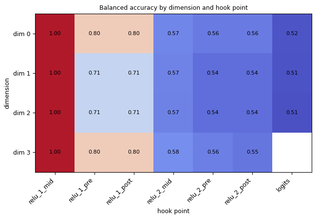How accurately can embedding sign in a dimension separate $x_0 > 0$ from $x_0 < 0$?

We can see that the first ReLU does this, since this is a very accurate predictor in relu_1_mid (and actually relu_0_post too, but I didn’t plot that). Another feature could be, how well does the sign of the embedding in a given dimension separate $x_1 > x_0$ from $x_0 > x_1$?

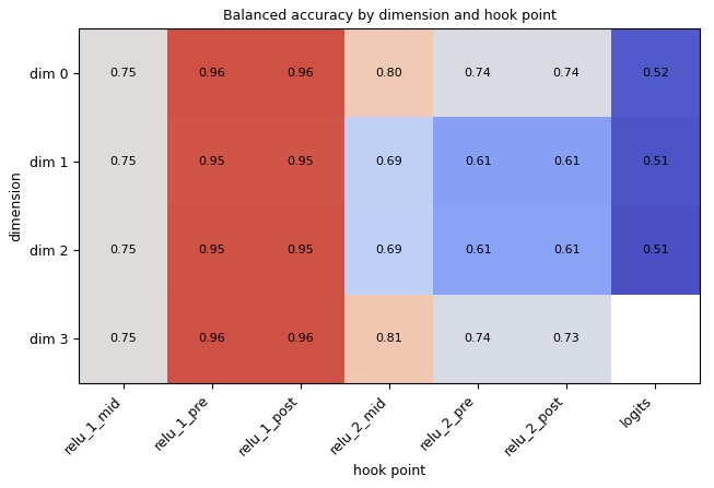How accurately can embedding sign in a dimension separate $x_0 > x_1$ from $x_1 > x_0$?

And we can see that relu_1_pre and relu_1_post does this. So those components very clearly encode such information. But, analyzing the separation dimension-by-dimension, based on a threshold ($0$) doesn’t work all the time - we got lucky so far. For example, we know that relu_2_post (1 linear transformation away from the logits) HAS to encode 2nd argmax information. I.E. the embeddings have to be linearly separable based on what their 2nd argmax is. Yet, there is no dimension in which a classifier based on thresholding (at $0$) achieves high accuracy at relu_2_post:

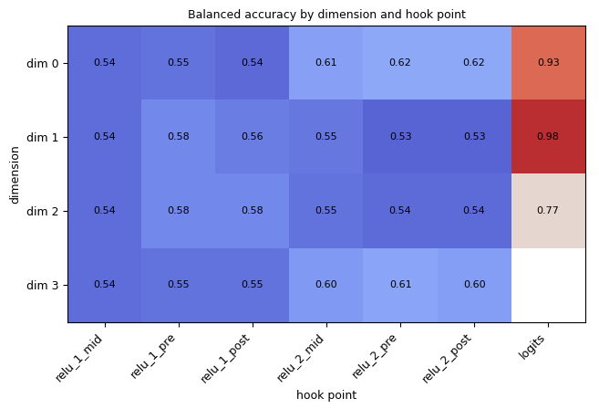How accurately can embedding sign in a dimension separate $\text{2nd argmax} = 1$ from $\text{2nd argmax} \neq 1$?

This is because there is no single dimension in which there exists a threshold that cleanly separates the various classes. The linear boundary cuts across 2 dimensions:

So we need to generalize this threshold from dimension-specific thresholds, to a general linear boundary. This is precisely a linear probe, which is a learnable logistic regression model that can learn a linear boundary in the entire hidden space, not just dimension-by-dimension.