I recently came across this paper by George Wang and Daniel Murfet at Timeaus that introduces the idea of “patterning” as the “dual problem” to mechanistic interpretability - i.e. if mech interp is about reverse engineering model internals, then patterning is the complementary question of how to influence training in order to produce a certain kind of model internals. I think it’s really interesting, but it strikes me that their paper could be more aggressively pared down to the essentials in order to really gain an intuition of how patterning works / is possible, so this is what this post will be about.
Introduction
First, they introduce a posterior of trained model weights $w$ given some dataset $D_n$ of size $n$:
\[\begin{align*} p(w \mid D_n) \end{align*}\]These weights $w$ are post-training weights, so $p(w \mid D_n)$ is implicitly also dependent on the model architecture and optimization parameters / algorithms. They further note that the shape of $p(w \mid D_n)$ reveals internal structural information of the model. For example, if there are redundancies in weights / circuitry, then perturbation of some weights will not matter so much to model performance, and hence there are groups of degenerate (“equivalent”) weight configurations. Another example of degeneracy is when a perturbation in a weight can be compensated for via coordinated perturbations in other weights.
Then, they claim that “structural information can be extracted by computing expectation values” of observables $\phi_i$ which one can design:
\[\begin{align*} \mu_i^n = \int \phi_i (w) p(w \mid D_n) dw \end{align*}\]$\phi_i$ could be a linear probe, an SAE, the “local learning coefficient $\lambda$” (introduced later), “susceptibilities $\chi$” (and another!), whatever - functions of the free parameter space of $w$. One can then collate these observable means into a vector of “structural coordinates”:
\[\begin{align*} \mu^n = \begin{bmatrix} \mu_1^n \\ \mu_2^n \\ \vdots \\ \end{bmatrix} \end{align*}\]Affordance
This paper is about studying the “affordances” (🙄) of these structural coordinates. What does that mean? Your guess is as good as mine.
First, the authors try to generalize $\mu^n$ to $\mu^\infty$, which they compute using the “annealed posterior”:
\[\begin{align*} p(w \mid D_\infty) \propto \frac{\varphi(w)}{\exp (n \beta L(w))} \end{align*}\]where:
\[\begin{align*} L(w) = \mathbb{E}_q [\ell(w)] \end{align*}\]is the “population loss”, where:
- $q$ is the data distribution (introducing $q$ makes sense since we’re trying to generalize $D_n$ to $D_\infty$).
- I assume $\beta$ is some hyperparameter.
- $\varphi$ is hthe prior density of $w$.
Matrix of Susceptibilities
Previously, we introduced $q$ as the data distribution, but now they say “let $h$ denote a vector of hyperparameters governing the data distribution (for instance, mixture weights [(???)] over a baseline distribution and a collection of probe distributions [(???)])”. Then:
\[\begin{align*} d \mu^\infty = \chi \cdot dh \end{align*}\]where $d$ refers to the total differential (i.e. first order approximation of $\partial$), and so $\chi$ is the Jacobian of $\mu^\infty$ w.r.t $h$. This is precisely the matrix of susceptibilities:
\[\begin{align*} \text{ } \\ \chi = \begin{bmatrix} \frac{\partial \mu_1}{\partial h_1} & \frac{\partial \mu_1}{\partial h_2} & \cdots & \frac{\partial \mu_1}{\partial h_k} \\ \frac{\partial \mu_2}{\partial h_1} & \frac{\partial \mu_2}{\partial h_2} & \cdots & \frac{\partial \mu_2}{\partial h_k} \\ \vdots & \vdots & \ddots & \vdots \\ \frac{\partial \mu_i}{\partial h_1} & \frac{\partial \mu_i}{\partial h_2} & \cdots & \frac{\partial \mu_i}{\partial h_k} \end{bmatrix} \end{align*}\]They continue: “the $ik$-entry $\chi_{ik}$ measures how the expectation of observable $\phi_i$ [(a.k.a. $\mu_i$, yes)] responds to an infinitesimal shift of the data distribution toward probe $k$” (which I’ve denoted $h_k$). Note that we still don’t know what these probes are like.
The Fundamental Equation of Patterning
So then, the natural question is, given that we would like to observe a target change in the observables $\mu^\infty$, what’s the minimum-norm intervention in the data distribution? It is just a rearrangement of the above equation:
\[\begin{align*} (d h)_\text{opt} = \chi^\dagger \cdot (d \mu^\infty)_\text{target} \end{align*}\]where $\chi^\dagger$ is the Moore-Penrose pseudoinverse. This, they call the Fundamental Equation of Patterning.
Producing Perceptible Changes
Summarizing from the last section, assuming that your observables $\phi$ and data hyperparameters $h$ work / are well designed (i.e. susceptibilities must be sensitive to internal structure), then $\chi$ is useful in telling you how to change $h$ in order to produce desired changes in $\phi$ (or $\mu^\infty$).
For example, Baker et. al found that “PC2 of the susceptibility matrix couples induction patterns in the data (roughly speaking, the right singular vector $v_2$) to the induction circuit in the weights (the left singular vector $u_2$),” and so up or down-weighting tokens with high $v_2$ magnitudes can accelerate or delay induction circuit formation. The unspoken part is that the design of $\phi$ and $h$ are crucial here, so we’ll just have to see how Wang and Murfet demonstrate this later on.
Another example is that if you know that there are multiple plausible internal structures that can solve the same problem (roughly, achieve the same small loss), you can use Patterning to select one of them in particular to be learnt. Wang and Murfet demonstrate this using a model trained on a bracket classification task.
Singular Learning Theory (SLT)
So far, we’ve mentioned that a key observable is the Local Learning Coefficient (LLC) $\lambda$, but we haven’t defined that. This necessitates an introduction to SLT, for it:
- Defines the LLC
- Provides mathematical framework (“annealed posteriors”, “free energy”) for susceptibilities.
Define “Singular” Statistical Model
A statistical model is simply something that models probability distributions
\[\begin{align*} p(y \mid x, w) \end{align*}\]by maximizing this (or some proxy, e.g. $\mathbb{E} p(y)$) w.r.t to $w$. A statistical model becomes singular when roughly, there are multiple solutions, or multiple ways to produce the same distribution. Neural networks are quite obviously singular.
Note: Another commonly cited explanation is when the Fisher Information (a Hessian) is degenerate (non-invertible; i.e. there exists some direction along which the likelihood has no curvature) at some $w$. But I find this to be insufficiently strict as a requirement, for zero curvature doesn’t mean that gradient of likelihood is 0, i.e. doesn’t mean that there are multiple parameter solutions to get the same probability distribution. However, the opposite is a quite a strong prerequisite: a model is definitely regular if the Fisher information matrix is positive definite.
Learning Coefficient
Consider a statistical model:
\[\begin{align*} p(y \mid x, w) \end{align*}\]with parameters $w \in W \subseteq \mathbb{R}^d$, which prior density $\varphi(w)$. Suppose also that the dataset $D_n = \{ (x_i, y_i) \}_{i=1}^n$ is drawn i.i.d. from a true distribution $q(x, y)$.
And define the empirical loss:
\[\begin{align*} L_n (w) = - \frac{1}{n} \sum_{I=1}^n \log p(y_i \mid x_i, w) \end{align*}\](basically just cross entropy loss), and the population loss:
\[\begin{align*} L(w) = - \mathbb{E}_{q(x, y)} \left[ \log p(y \mid x, w) \right] \end{align*}\]Define the volume:
\[\begin{align*} \text{vol}(\epsilon) = \int_{L(w) < L(w^\star) + \epsilon} \varphi (w) \end{align*}\]where $w^\star$ is the global minimizer of $L$. Intuitively speaking, this is the probability mass (according to $\phi$) over all $w$ that produce “small enough” $L(w)$. The learning coefficient is then a measure of how fast this volume shrinks:
\[\lambda = - \lim_{\epsilon \rightarrow 0^+} \log_2 \left[ \frac{\text{vol}\left( \frac{\epsilon}{2}\right)}{ \text{vol} (\epsilon)} \right]\]Note: There is probably heavy theory behind the construction using $\log_2$ and the claim that in regular models (where $w^\star$ is unique and the Hessian is non-degenerate), $\lambda = d/2$ where $d$ is the parameter dimension, but this is not relevant for our discussion.
A high $\lambda$ means that from $\epsilon \rightarrow \epsilon / 2$, the volume decreases by relatively much, while a low $\lambda$ means that the volume doesn’t decrease by that much. I think of this by visualizing a highly pointy function versus a relatively smooth / bowl-shaped one, and noticing that the relative sizes of the 2 cylinder volumes are much more comparable for the low $\lambda$ function:
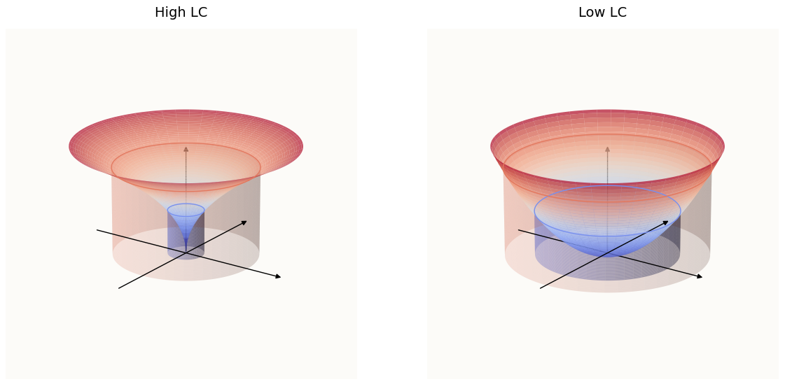 Pointier (high LC) versus Bowl / Flatter (low LC). [0, 0] is the minimizer; vertical axis is $\varphi$.
So basically, $\lambda$ is conceptually similar to the Fisher Information $\mathcal{I}(w)$. With the learning coefficient defined, the LLC is just a local version of that. And since there are assumed to be multiple local minima, you also have to specify which local minimum $w^\star$ it is, so it is denoted as $\lambda (w^\star)$.
Posterior $p(w \mid D_n)$
The next concept introduced is the Bayesian posterior probability of a small neighborhood $\mathcal{U}$ around a local minimum $w^\star$:
\[\begin{align*} p_n(\mathcal{U}) = \frac{Z_n(\mathcal{U})}{Z_n(\mathcal{W})} \end{align*}\]where
\[\begin{align*} Z_n(\mathcal{U}) = \int_{\mathcal{U}} \exp \left( -n L_n(w)\right) \varphi (w) dw \end{align*}\]Derivation of Posterior
Why is this correct? Starting from Bayes’ theorem, we have:
\[\begin{align*} p(w \mid D_n) \propto p(D_n \mid w) \varphi (w) \end{align*}\]Playing with $\exp$, $\log$, and substituting in the definition of empirical loss $L_n(w)$ defined above, the likelihood of i.i.d. data is:
\[\begin{align*} p(D_n \mid w) & = \prod_{i = 1}^n p(y_i \mid x_i, w) \\ & = \exp \left( \sum_{i=1}^n \log p( y_i \mid x_i, w) \right) \\ & = \exp \left( -n L_n(w) \right) \end{align*}\]So we have the posterior equals:
\[\begin{align*} p_n(\mathcal{U}) = \frac{\int_{\mathcal{U}} \exp \left( -n L_n(w) \right) \varphi(w)}{Z_n(\mathcal{W})} \end{align*}\]where the denominator is just a normalizing constant.
Free Energy
They next introduce the “Local Free Energy $F_n(\mathcal{U})$”:
\[\begin{align*} F_n(\mathcal{U}) = - \log Z_n(\mathcal{U}) \end{align*}\]This is a measure of how much posterior mass is in the neighborhood $\mathcal{U}$:
- Large posterior mass in $\mathcal{U} \Longleftrightarrow$ low $F_n(\mathcal{U})$
- Small posterior mass in $\mathcal{U} \Longleftrightarrow$ large $F_n(\mathcal{U})$
They then cite the asymptotic ($n \rightarrow \infty$) expansion from Watanabe, 2009:
\[\begin{align*} F_n(\mathcal{U}) = n L_n(w^\star) + \lambda (w^\star) \log n - (m(w^\star) - 1)\log \log n + O_p(1) \end{align*}\]where “$m(w^\star)$ is the multiplicity, a secondary geometric invariant.”
Derivation
Lmao I dunno mate Claude gave me crap. I’m willing to just say this is a result from Watanabe and move on.
Bayesian Inference Prefers Lower Free Energy
The paper compares two local minima $w_A^\star$ and $w_B^\star$ with neighborhoods $\mathcal{U}$ and $\mathcal{V}$ via this difference of free energy:
\[\begin{align*} \log \frac{p_n (\mathcal{U})}{p_n (\mathcal{V})} & = F_n(\mathcal{V}) - F_n(\mathcal{U}) \\ & = \Delta L_n \cdot n + \Delta \lambda \cdot \log n + O_p (\log \log n) \end{align*}\]And they note that when the 2 local minima achieve the same loss, then the difference in free energy (or ratio of posteriors) depends entirely on $\Delta \lambda$. They then make the claim that “among equal-loss solutions, the posterior favors those with lower LLC.” I.E. they mean that the posterior for the lower LLC optimum is actually higher than that of the higher LLC optimum.
How is it possible that a local optimum can be favored over another despite producing equal loss? My understanding is that the heavy lifting is done by choosing the prior distribution $\varphi (w)$ ($\lambda(w)$ does depends on this afterall), and by relating the posterior to $\lambda(w)$. It remains to be seen how this is chosen well.
Estimating the LLC
Since the LLC is the ratio of volumes, and these volumes are integrals of the prior $\varphi$ over parameter space and have no analytical solution, they use prior work to estimate the LLC:
\[\begin{align*} \hat{\lambda} (w^\star) & = n \beta \left[ \mathbb{E}^\beta_{w \mid w^\star, \gamma} \left[ L_n(w) \right] - L_n(w^\star) \right] \end{align*}\]where the “expectation is w.r.t a localized tempered posterior” (Watanabe, 2013):
\[\begin{align*} p(w; w^\star, \beta, \gamma) & \propto \exp \left\{ -n \beta L_n(w) - \frac{\gamma}{2} \|w - w^\star \|^2 \right\} \end{align*}\]where these are the hyperparameters:
- $\beta$ is the inverse temperature
- $\gamma$ is the localization strength
Derivation of Localized Tempered Posterior
Starting with the definition of posterior (similar to our derivation in Derivation of Posterior):
\[\begin{align*} p(w \mid D_n) & \propto p(D_n \mid w) \varphi (w) \\ & \propto \prod_{i=1}^n p(y_i \mid x_i, w) \varphi(w) \end{align*}\]Then, an inverse temperature ($\beta < 1$) modification is applied to the likelihood term to flatten the likelihood distribution:
\[\begin{align*} p(w \mid D_n) & \prod_{i=1}^n p(y_i \mid x_i, w)^\beta \varphi(w) \\ & \propto \exp \left( \sum_{i=1}^n \beta \log p(y_i \mid x_i, w) \right) \varphi(w) \\ & \propto \exp \left( -n \beta L_n(w) \right) \varphi(w) \end{align*}\]A localization modification is applied to the prior term to assume that $\varphi(w)$ is Gaussian centered at $w^\star$:
\[\begin{align*} p(w \mid D_n) & \propto \exp \left( -n \beta L_n(w) \right) \cdot c_G \cdot \exp \left( - \frac{(w - w^\star)^2}{2 \sigma^2} \right) \\ & \propto \exp \left( -n \beta L_n(w) - \frac{(w - w^\star)^2}{2 \sigma^2} \right) \end{align*}\]where $c_G$ is the normalization factor for the Gaussian PDF. Then, the localization strength parameter is applied to replace $\sigma$:
\[\begin{align*} p(w \mid D_n) & \propto \exp \left( -n \beta L_n(w) - \frac{(w - w^\star)^2}{2 (1 / \sqrt{\gamma})^2} \right) \\ & \propto \exp \left( -n \beta L_n(w) - \frac{\gamma}{2} \| w - w^\star \|^2 \right) \end{align*}\]As is the standard result, the minimization of the L2 loss term can be interpreted as:
- Wanting to achieve a tighter fit and minimization of Gaussian noise; hence $\uparrow \lambda \Rightarrow$ smaller std. deviation in the Gaussian prior term.
- Higher weight on the L2 loss penalty (hence also encouraging tighter fit)
Widely Applicable Bayesian Information Criterion (WBIC)
Introduced in the aforementioned (WBIC paper (Watanabe, 2013)) is the eponymous WBIC, which expands into a function of $\lambda$:
\[\begin{align*} \text{WBIC} & = \mathbb{E}_w^\beta \left[ n L_n (w) \right], \space \beta = \frac{1}{\log n} \end{align*}\]Watanabe’s main theorem shows that:
\[\begin{align*} \text{WBIC} & \simeq n L_n (w^\star) + \lambda \log n \end{align*}\]Now rearrange this for $\lambda$:
\[\begin{align*} \lambda & \approx \frac{\text{WBIC} - n L_n(w_0)}{\log n} \\ & = \frac{\mathbb{E}_w^\beta \left[ n L_n (w) \right] -n L_n(w^\star)}{\log n} \\ & = n \beta \left[ \mathbb{E}_w^\beta \left[ L_n (w) \right] - L_n(w^\star) \right] \end{align*}\]Which is exactly the LLC estimator. The only difference is we use $\mathbb{E}_{w \mid w^\star, \gamma}^\beta$ to denote that the expectation is using the localized tempered posterior.
Estimating Susceptibility
Remember that the susceptibility is roughly the first derivative of an observable w.r.t some dataset hyperparameter (probe). The observable in this case can be something as general as posterior probability of the parameters or the loss of the model with those parameters.
Shifting their discussion concretely to the LLM, they define
- Sequence models $p(y \mid x, w)$ that predict
- Tokens $y \in \Sigma$ given some
- Context $x \in \Sigma^k$ of length $1 < k \leq K$ where $K$ is the max context length, that are specifically
- a Transformer with a vector of weights $w \in W$.
They also define a product decomposition $W = U \times C$ (think of this as segmenting the vector $w$ into 2 disjoint sets), which is useful for thinking of the weights as a sum of component-wise weights.
Define further:
- Dataset $D_n = { (x_i, y_i) }_{i=1}^n$ drawn i.i.d. from
- True distribution $q(x, y)$
- The standard losses:
- Sample negative-log-likelihood (NLL) $\ell_{xy} (w) = - \log p(y \mid x, w)$
- Mean NLL (a.k.a. Cross Entropy Loss) $L_n(w) = \frac{1}{n} \sum_{i=1}^n \ell_{xy}(w)$.
We can define an observable that attempts to measure the “slack” a current $w$ has, i.e. if you were to freeze all the weights except for a component in question $C$, how would the posterior or loss change when you vary $c$ around its current location? To do this, they define this quantity:
\[\begin{align*} \phi_C (w) = \delta (u - u^\star)\left[ L(w) - L(w^\star) \right] \end{align*}\]Where $\delta$ is the Dirac delta (think of it as an indicator variable that switches on only when $u$ is at its current trained location $u^\star$). So, $\phi_C(w)$ measures the difference in loss when you vary $c$ in $w = (u^\star, c)$. In reality, this quantity can be any similarly useful quantity, so they call this a “generalized function”.
To capture “slack”, one can use the expectation $\langle \phi_C(w) \rangle_\beta$.
Deriving the Expectation
The annealed posterior (seems to me to be the same posterior as in Derivation Of Posterior) is:
\[\begin{align*} p_n^\beta (w) & = \frac{\exp \left\{ -n \beta L (w) \right\} \varphi(w)}{Z_n^\beta} \\ \text{where } Z_n^\beta & = \int \exp \left\{ -n \beta L(w) \right\} \varphi(w) dw \end{align*}\]The only difference is that they did not expand $\varphi(w)$, which I assume is Gaussian at local minima. So then the expectation is:
\[\begin{align*} \langle \phi \rangle_\beta = \int \phi(w) p_n^\beta (w) dw \end{align*}\]Susceptibility of Posterior Expectation
The susceptibility of posterior expectation to a perturbation of data parameter $h$ is intuitively just the derivative:
\[\begin{align*} \chi = \frac{1}{n \beta} \frac{\partial}{\partial h} \langle \phi \rangle_{\beta, h}\bigg|_{h=0} \end{align*}\]There’s an additional $\frac{1}{n \beta}$ multiplicative factor here because it becomes convenient with later steps.
Per-Token Susceptibility
Define the per-token susceptibility of component $C$ for $(x, y)$ as:
\[\begin{align*} \chi_{xy}^C = - \text{Cov}_\beta \left[ \phi_C, \ell_{xy} (w) - L(w)\right] \end{align*}\]Deriving the Susceptibility
The derivation of the above expression is just straightforward differentiation of $\phi$, but just for my future reference:
\[\begin{align*} \langle \phi \rangle_{\beta, h} & = \frac{\int \phi(w) \exp \left\{ -n \beta L_h(w) \right\} \varphi (w) dw}{\int \exp \left\{ -n \beta L_h(w) \right\} \varphi(w) dw} \end{align*}\]Derivative of numerator:
\[\begin{align*} \frac{\partial \text{ numerator}}{\partial h} = -n \beta \int \phi (w) \left( \frac{\partial L_h (w)}{\partial h} \right) \exp \left\{ -n \beta L(w) \right\} \varphi(w) dw \end{align*}\]Derivative of denominator:
\[\begin{align*} \frac{\partial \text{ denominator}}{\partial h} = -n \beta \int \left( \frac{\partial L_h (w)}{\partial h} \right) \exp \left\{ -n \beta L(w) \right\} \varphi(w) dw \end{align*}\]Apply quotient rule,