Thinking about how Sparse Auto-encoders (SAEs) aim to learn a sparse over-complete basis (where you are trying to triangulate a larger number of sources than you have signals; e.g. you only have 8 microphones in the room, but there are 20 speakers) got me thinking about Independent Component Analysis again. In particular, I wanted to see if I could articulate a mapping between ICA and SAEs. This would provide a more mathematical framework for thinking about SAEs. I do so in this post by walking through this paper: Lewicki and Sejnowski
As a reminder, SAEs are Anthropic’s way of trying to extract mono-semantic features (which are directions in a model’s latent space that correspond to interpretable concepts like “French aristocracy,” “sycophancy,” “Chemistry measurement apparatus,” etc.). The main idea behind SAEs is that all data latents are simply a sparse combination of a very large dictionary of feature vectors. ICA is yet another way to extract “archetypical” features from a dataset, but ICA is driven by assumptions about the statistical distribution of these archetypical features, and not specifically sparsity, although they can coincide.
In this post, I will:
- Intuitively trace through the derivation of Lewicki & Sejnowski
- Compare ICA with SAEs
- Implement ICA, demonstrate problems that Lewick & Sejnowski did not mention, and add refinements
- (Maybe) apply ICA to Language Models / Vision Models to see what I find
Lewicki and Sejnowski
This paper investigates “using a Laplacian prior” to learn “representations that are sparse and [a] non-linear function of the data” as a “method for blind source separation of fewer mixtures than sources”.
Motivations
- Overcomplete representations “(i.e. more basis vectors than input variables), can provide a better representation, because the basis vectors can be specialized for a larger variety of features present in the entire ensemble of data”
- But, “a criticism of overcomplete representations is that they are redundant, i.e. a given data point may have many possible representations”
- This paper is about imposing a prior probability of the basis coefficients which “specifies the probability of the alternative representations”. I’m not sure I understand this for now.
Problem Setup
\[\begin{align*} x & = As + \varepsilon \end{align*}\]where $A \in \mathbb{R}^{m \times n}, m < n$. $x$ is the observation (short vector), while $s$ is the hidden “true” source signal vector. Further, they assume “Gaussian additive noise so that $\log P(x \mid A, s) \propto - \lambda (x - As)^2 / 2$.” Whatever 🙄:
\[\varepsilon \sim \mathcal{N} \left(0, \frac{1}{\lambda}\right)\]They further define a “density for the basis coefficients, $P(s)$, which specifies the probability of the alternative representations. The most probable representation, $\hat{s}$, is found by maximizing the posterior distribution:”
\[\hat{s} = \max_s P(s \mid A, x) = \max_s P(s) P(x \mid A, s)\]Firstly, they mean to say:
\[\hat{s} = \text{argmax}_s P(s \mid A, x) = \text{argmax}_s P(s) P(x \mid A, s)\]And I should note that this is simply Bayes’ rule being applied. In this case, $P(s)$, a.k.a the prior, has been hydrated out and assumed to be Laplacian.
Approaches considered
They considered these optimization approaches:
- Find $\text{argmax}_s P(s \mid A, x)$ by using the gradient of the log posterior ($\log P(s \mid A, x)$).
- Use linear programming methods to find $A$ and $s$ to maximize $\text{argmax}_s P(s \mid A, x)$ while minimizing $\mathbf{1}^\top s = |s|_1$. This is exactly equivalent to the objective of SAEs.
Learning Objective
“The learning objective is to adapt $A$ to maximize the probability of the data which is computed by marginalizing over the internal state:”
\[\begin{align*} P(x \mid A) & = \int P(s) P(x \mid A, s) \text{ } ds \end{align*}\]This, I understand. A helpful note is that $s$ is distributed around some mean ($\hat{s}$), and that distribution is usually Gaussian, but in this paper, they propose for it to be Laplacian. Remember also that while $s \sim \text{Laplacian}$, the noise $\varepsilon$ in the data is still Gaussian.
They continue: “this integral cannot be evaluated analytically but can be approximated with a Gaussian integral (hence why it’s usually Gaussian) around $\hat{s}$, yielding:”
\[\begin{align*} \log P(x \mid A) \approx \text{const.} + \log P(\hat{s}) - \frac{\lambda}{2}(x - A\hat{s})^2 - \frac{1}{2} \log \text{det} H \end{align*}\]“where $H$ is the Hessian of the log posterior at $\hat{s}$.” This, I did not understand, but I was able to trace through the derivation with Claude’s help and so I’ll write it down before it’s lost once again to the ether. The following subsections are me banging out the math and explaining it, so feel free to skip to just before Comparison with SAEs where the final update rule is stated.
Derivation of Approximation
First, we denote the log of the integrand as $f(s)$:
\[\begin{align*} f(s) & = \log P(s) + \log P(x \mid A, s) \\ \therefore P(x \mid A) & = \int e^{f(s)} \text{ } ds \end{align*}\]We know that the mean of a Gaussian (and Laplacian for that matter) distribution has the maximum probability density. This is a useful fact about $\hat{s}$, which we will try to incorporate by expressing $f(s)$ in terms of $f(\hat{s})$ using the Taylor expansion:
\[\begin{align*} f(s) & \approx f(\hat{s}) + \nabla f(\hat{s})^\top \left(s - \hat{s} \right) + \frac{1}{2} \left( s - \hat{s} \right)^\top H \left( s - \hat{s}\right) \end{align*}\]Since, by Bayes rule,
\[\begin{align*} \log P (s \mid x, A) & = \log P(s) + \log P(x \mid A, s) - \log P(x \mid A), \\ \Rightarrow \log P(s \mid x, A) & \propto \log P(s) + \log P(x \mid A, s) = f(s) \end{align*}\]Since $\hat{s} = \text{argmax}_s P(s \mid x, A)$, this also means that $f(s)$ is maximized at $\hat{s}$. Hence, $\nabla f(\hat{s})$ at $\hat{s}$ is $0$. Therefore:
\[f(s) \approx f(\hat{s}) + \frac{1}{2}\left( s - \hat{s} \right)^\top H \left(s - \hat{s} \right)\]Substituting back into the integral, we have:
\[\begin{align*} P(x \mid A) & \approx \int e^{f(\hat{s})} e^{\frac{1}{2}(s - \hat{s})^\top H (s - \hat{s})} \text{ } ds \\ & = e^{f(\hat{s})} \int e^{-\frac{1}{2}(s - \hat{s})^\top K (s - \hat{s})} \text{ } ds \end{align*}\]Where $K = -H$. Crucially, the second term is a Gaussian integral, with a known solution below.Note that because $H$ is the Hessian of a concave quadratic, $H$ is negative definite, and has a positive determinant if $s$ is even-dimensional, and negative determinant if $s$ is odd-dimensional. Since we’re using $K = -H$, this is not a problem anymore because $K$ is positive semidefinite and has a non-negative determinant.
\[\begin{align*} \int e^{-\frac{1}{2}(s - \hat{s})^\top K (s - \hat{s})} \text{ } ds & = \sqrt{\frac{(2 \pi)^d}{| K |}} \end{align*}\]Where $|K |$ is the determinant of $K$. Therefore:
\[\begin{align*} P(x \mid A) & \approx e^{f(\hat{s})} \int e^{-\frac{1}{2}(s - \hat{s})^\top K (s - \hat{s})} \text{ } ds \\ & = e^{f(\hat{s})} (2 \pi)^\frac{d}{2} \cdot | K | ^{-\frac{1}{2}} \\ \Rightarrow \log P(x \mid A) & = f (\hat{s}) + \frac{d}{2} \log (2 \pi) - \frac{1}{2} \log |K| \\ & = \log P(\hat{s}) + \log P(x \mid A, \hat{s}) + \frac{d}{2} \log (2 \pi) - \frac{1}{2} \log |K| \\ \end{align*}\]At this point, we pretty much have what we want. We just have to note that for the $\log P(x \mid A, \hat{s})$ term, since Gaussian PDF is given by some scalar multiple of $\exp(-(x - \mu)^2)$, we simply have:
\[\begin{align*} \log P(x \mid A, s) = -k \left( x - A \hat{s} \right)^2 + \text{const} \end{align*}\]And further noting that the $\frac{d}{2} \log (2 \pi)$ term is a constant, we have our approximation:
\[\begin{align*} \log P(x \mid A) \approx \text{const} + \log P (\hat{s}) - k(x - A\hat{s})^2 - \frac{1}{2} \log |K| \end{align*}\]Where $|K|$ is explicitly the absolute value of the determinant of $H$, and not the determinant of $H$, as the paper suggests.
Learning Rule
As with normal gradient ascent algorithms, our learning rule is to update $A$ with $A + \Delta A$, where $\Delta A$ is the gradient of the maximization objective, in this case: $\log P(X \mid A)$. I’ll skim the derivation of the learning rule:
First term:
\[\begin{align*} \nabla_A \log P(\hat{s}) & = \nabla_{\hat{s}} \log P(\hat{s}) \cdot \nabla_{A} \hat{s} \\ \end{align*}\]Things to note / denote:
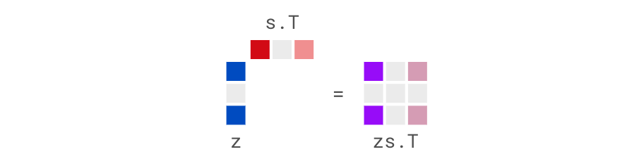
- $z = \nabla_s \log P(s)$
- $W \approx A^{-\top}$, in the sense that rows of $W^\top$ corresponding to non-zero $s$ indices are the same as those of $A^{-\top}$, and hence $A^\top W^\top = I$
So first term becomes (I don’t fully follow the assumptions that allow the conflation of $\hat{s}$ and $s$, and $A^{-\top}$ and $W^\top$, but I can big-picture follow the chain rule):
\[\begin{align*} \nabla_A \log P(\hat{s}) & = -W^\top z s^\top \end{align*}\]Second term:
\[- k (x - A\hat{s})^2\]This is simply a noise term, and the Gaussian noise is irreducible error. There’s no gradient w.r.t $A$ from this term.
Third term: I’m not even going to trace through the derivation for this one:
\[\begin{align*} \nabla_A \frac{1}{2} \log \text{det} (H) & = \lambda A H^{-1} - 2W^\top y \hat{s}^\top \end{align*}\]Where $y$ “hides a computation involving the inverse Hessian… It can be shown that if $ \log P(s)$ and its derivatives are smooth, $y$ vanishes for large $\lambda$.”
Putting it together:
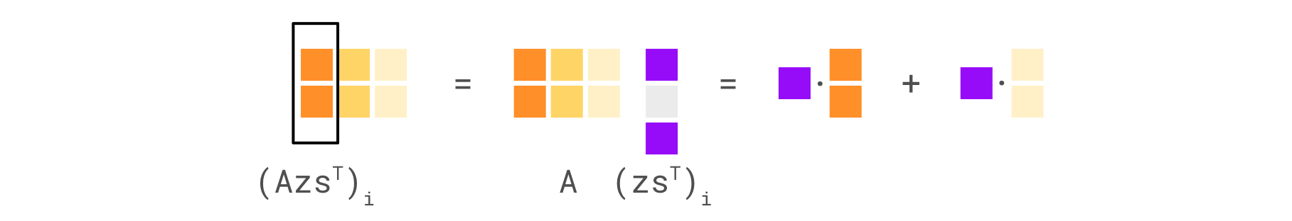
\[\begin{align*} \nabla_A \log P(x \mid A) & = -W^\top z s^\top - \lambda AH^{-1} + 2A y s^\top \\ & = -W^\top z s^\top - \lambda AH^{-1} \text{ (last term vanished)} \end{align*}\]The authors then choose to normalize this by $AA^\top$, which they do not explain, and I do not understand. A wild guess is that usually, $AA^\top$ captures geometry of $A$, in the sense that $AA^\top$’s eigenvalues will tell you the stretching factor in each dimension, and hence the “variance” in each dimension, and you might hence want to scale up your updates accordingly.
\[\begin{align*} AA^\top \nabla_A \log P(x \mid A) & = A z s^\top - \lambda A A^\top AH^{-1} \end{align*}\]Below, we ran into some altercations involving $AA^\top$. In particular, multiplying our update by $AA^\top$ gave us better optimization behavior, but I still do not know why. If you had thoughts about this, I would appreciate if you shared them!
More assumptions: if $\lambda$ is large (low noise, as large $\lambda \Rightarrow$ low standard deviation), “then the Hessian is dominated by $\lambda A^\top A$, and we have”:
\[\begin{align*} - \lambda A A^\top AH^{-1} & = \lambda A A^\top A (A^\top A + B)^{-1} \approx -A \end{align*}\]And we have this final update rule:
\[\begin{align*} A & := - \alpha (A z s^\top + A) \end{align*}\]Comparison with SAEs
vs SAEs
Denoting a simplified SAE encoder function as:
\[\begin{align*} s & = \text{ReLU} (W_\text{enc}x + b_{enc}) \\ x' & = W_\text{dec} s + b_{dec} \end{align*}\]Both SAEs and ICA are supposing that the data is compressed and are trying to do decompression, but we can already see 2 differences. The first is that relying on $\text{ReLU}$ to hydrate your individual features presupposes that your data is sparse. In particular, because the latent space will always look something like this:
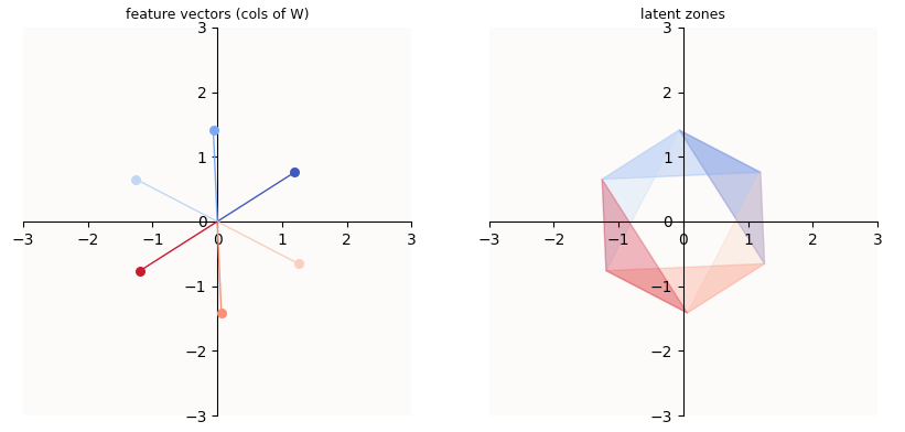 “Superposition - An Actual Image of Latent Spaces”
You can notice that not all types of data vectors $x$ can be reconstructed. If $x$ is one-hot, you’re in good shape, because the embeddings of $x$ ($s$) will sit along its feature vector and be only in the activation zone of that one feature. However, if $x$ is two-hot, then the 2 features that are active better be one of the 6 pairs for which there is an overlap of those 2 features’ activation zones (corresponding to the edges of the hexagon in the latent zone plot). If $x$ is three-hot, you’re out of luck, because there isn’t a zone in the latent where the latent zones of 3 features overlap. In a 3D latent, such zones would correspond to a face, but you can see how density quickly hinders your reconstruction ability.
ICA does not rely on $\text{ReLU}$ to decompress features. ICA relies on statistical arguments of minimizing covariance of features and maximizing the a posteriori likelihood of the data given some prior, which brings us to the second difference.
The update rule of Lewicki and Sejnowski has $z$ in it. Remember that $z = \nabla_s \log P(s)$. $P(s)$ in particular, is defined by the user; in this case, it is Laplacian, simply because we said so. This variant of ICA allows us to build in explicit hypotheses about the distribution of “true feature” / source signal activations (coefficients) as our prior.
Looking at activation histograms that Anthropic has generated, I’d say that the Laplacian distribution is a reasonable approximation to a large number of feature activation distributions, and that there is a possible research question worth exploring: what if we used Lewicki and Sejnowski to try and find features instead of SAEs?
Experiment Log
Let’s try to do just that then! First, we’ll try to implement Lewick & Sejnowski in a toy dataset. This toy dataset will allow us to really understand the technique, its limitations, and make small modifications to it (such as allowing only positive coefficients) before trying to apply it to large models.
E1. Data Generation
Our goal is to have data that looks like this:
 Desired Dataset (from “Examples” of Lewicki & Sejnowski)
A Laplacian prior does not give a dataset that looks like this. It gives a symmetric spherical dataset, much like a multivariate Gaussian. I then found that they wrote that “the elements of $s$ [are] distributed according to an exponential distribution with unit mean.” I was able to recover something like that using an exponential prior:
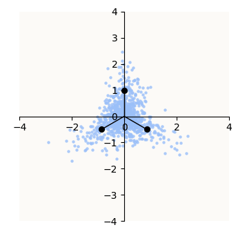 Exponential Prior Dataset ($\lambda = 0.5$, i.e. mean of 2)
They further state that “identical results were obtained by drawing $s$ from a Laplacian prior (positive and negative coefficients).” This is incredible, because it means that the update rule is readily applicable to the feature (non-negative coefficients) extraction setting. And indeed, the PDF for each half of the Laplace distribution belongs to the same family of distributions as the PDF of the exponential distribution. Their shapes are exactly the same up to a scaling factor, and the scaling factor is completely irrelevant in the context of gradient descent! 😄 😄
E2. Solving for $\hat{s}$ Given a Fixed $A$
Remember that the update rule is:
\[A := - \alpha (A z \hat{s}^\top + A)\]So first, we have to solve for $\hat{s}$. The paper states that “coefficients were solved using BPMPD,” where BPMPD is a primal-dual interior point algorithm. Sorry Stephen Boyd, as much as I loved convex optimization, I’m not about to re-write a convex optimization algorithm. We will instead using good old gradient descent.
Given a fixed $A$ and a data matrix $X \in \mathbb{R}^{n \times p}$, we shall find $\hat{s}$. Remember that this is the definition of $\hat{s}$:
\[\hat{s} = \text{argmax}_s P(s \mid A, x) = \text{argmax}_s P(s) P(x \mid A, s)\]Log it:
\[\hat{s} = \text{argmax}_s \log P(s \mid A, x) = \text{argmax}_s \left\{ \log P(s) + \log P(x \mid A, s) \right\}\]The first term is easy to compute; just plug $s$ into the equation for the Laplace Distribution PDF:
\[\begin{align*} P(s) & = \text{(Some constant)} \exp \left( - \frac{\|s - (\mu_s = 0)\|_1}{\lambda_\text{Laplace}} \right) \\ \log P(s) & = \text{(Some constant) } - \frac{\|s\|_1}{\lambda_\text{Laplace}} \end{align*}\]The second term is harder. We know that the noise model is:
\[x | A, s \sim \mathcal{N}(As, \sigma^2 I)\]Therefore, the likelihood and log-likelihood are:
\[\begin{align*} P(x \mid A, s) &= (2 \pi \sigma^2)^{-\frac{m}{2}} \exp \left(-\frac{\|x - As\|_2^2}{2 \sigma^2} \right) \\ \log P(x \mid A, s) &= - \frac{m}{2} \log (2 \pi \sigma^2 ) - \frac{\|x - As\|_2^2}{2 \sigma^2} \end{align*}\]where $m$ is the signal (measurement) dimensionality. Putting these together, we get the LASSO objective, aka minimize:
\[\begin{align*} \mathcal{L}_s = \frac{\|x - As\|_2^2}{2 \sigma^2} + \frac{\|s\|_1}{\lambda_\text{Laplace}} \end{align*}\]This looks similar to the SAE cost function:
\[\mathcal{L}_\text{SAE}(A, s) = \text{MSE}(x, As) + \lambda_\text{sparsity} \|s\|_1\]But there are 2 main differences. In training SAEs, the optimization is done on $A$ and $s$ simultaneously, whereas in ICA, the optimization is done on $s$ first to find $\hat{s}$. Then, in addition to this, we still have to find $z$, to optimize $A$. These are indeed not isomorphic, not even conceptually.
Implementing the learning of $\hat{s}$ is rather straightforward, with the update equation simply being:
\[s := \text{ReLU}(s - \nabla_s \mathcal{L}_s)\]E3 Updating $A$ given $\hat{s}$
The update equation here is simply from the paper:
\[A := - \alpha A(z s^\top + I)\]Since $z = \nabla_s \log P(\hat{s})$, and $s \sim \text{Laplace}(0, \lambda)$, it turns out that $z$ is simply $\frac{1}{\lambda} \text{sign}(\hat{s})$. The update to $A$ is very problematic, and while I was able to get perfect learning behavior when initializing $A$ with a perturbed version of $A$:
There is a failure mode where the updates to $A$ fall into a runaway regime, resulting in exploding losses:
I’ve noticed that this happens when the learning rate ($\alpha$) is unsuitable (either too high, or no learning rate scheduler is used), and / or the initialization of $A$ is random:
Solving this problem / figuring out why this happens is crucial before trying to implement this in real language models to extract features, because our features are definitely going to be randomly initialized, and we don’t know how many features (columns) to provision for in $A$.
E4 Re-Examining the Update Rule
\[A := - \alpha A(z \hat{s}^\top + I)\]Being forced to stare at this update rule, I now notice that this update rule doesn’t seem to be proportional to the error the way neural-network / general loss back-propagation update rules usually are. In particular, consider the case of perfect data reconstruction:
- $z$ is still $\frac{1}{\lambda} \text{sign}(\hat{s})$, as is the case in imperfect reconstruction
- $\hat{s}^\top$ is still $\hat{s}^\top$; it’s not as if $\hat{s}$ vanishes as reconstruction error vanishes
- $I$ is still $I$
I wonder if this is a problem. In particular, perhaps the fact that we’re throwing in a $\text{ReLU}$ to make all the source feature coefficients ($\hat{s}$) non-negative is disrupting a symmetry that is crucial to the update rule working.
E4.1 Laplace vs Exponential
So, I tested removing the $\text{ReLU}$ that was applied to $\hat{s}$ after each iteration of learning $\hat{s}$. This effectively makes it such that $s \sim \text{Laplace}$ instead of $s \sim \text{Exponential}$. These are the results I got:
There’s a new problem where the features recovered in $A$ do not rotate to align with the true features anymore. There are 2 observations that make it unclear why exactly achieving perfectly alignment is dis-preferred here:
- Imagine that $A$ were $A_\text{true}$, but flipped vertically. If we allowed negative coefficients, we can achieve the same sparsity that is achievable by $A_\text{true}$. All the coefficients just have to have the opposite sign. There is no incentive to rotate. However, this is not true if $A$ were some general rotation of $A_\text{true}$, and not exactly vertically flipped, as is the case shown above.
- Sparsity can be reduced by increasing the magnitude of the features in $A$.
In any case, this seems to be introducing a new problem, so it’d be more fruitful it seems to look elsewhere.
E4.2 Gaussian Noise?
In my prior experiments, I did not add Gaussian noise to $x$, as the paper supposes. Multiple times in the paper they allude to noise being crucial:
- “Recently Olshausen and Field (1996) presented an algorithm that allows an overcomplete basis to be learned. This algorithm […], including a tendency to breakdown in the case of low noise levels and when learning bases with higher degrees of overcompleteness.”
- Many times in the paper they simply write that they are assuming low noise.
So… I just added Gaussian Noise:
\[x = As + \left(\varepsilon \sim \mathcal{N}(0, 0.05^2) \right)\]Didn’t work; still exhibited the increase of error past a certain point:
E4.3 Normalizing by $(AA^\top)^{-1}$
A collaborator, Simon, then told me that perhaps I was missing the $(AA^\top)^{-1}$ term. I’m not sure where in the paper he got this from; the only place I saw a $AA^\top$ was equation $(5)$:
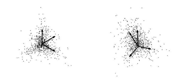
\[\Delta A = A A^\top \nabla \log P(x \mid A) \approx -A (z \hat{s}^\top + I)\]But! Analyzing the update equation, I found that it makes sense to normalize the update magnitudes by… what I interpret as the Mahalanobis distances of $A$. So, I added it in, and to see its affects, I plotted out the directions and relative magnitudes of the update terms (partial: $-Az\hat{s}^\top$, as well as full: $-A(z \hat{s}^\top + I)$) before and after adding the normalization term:
Before normalization:
How do we interpret the diagrams on the bottom row? Each arrow represents the quantity in the chart’s title, and the arrow’s color represents which data-point (there are only 3 of them here) is contributing that. The black arrow represents the sum contribution. The magnitude of the arrow is then rescaled for legibility. The colors of the data point reconstructions are a weighted sum of RGB, where the coefficient for each of the R, G, and B, are the values in $\hat{s}$ for that data point.
You can see that before normalization, $-Az\hat{s}^\top$ and $-Az\hat{s}^\top - A$ are not at all proportional to the error between the predicted $A$ and the true $A_\text{true}$. In fact, it seemed like the opposite, where the closer $A$ was to $A_\text{true}$, the bigger the updates, causing oscillation problems. Eventually, a too large step is taken and one or multiple of the features become dead ($\hat{s}_i$ is never $> 0$ for some feature $i$) and the error explodes.
After normalization:
You can see that now, the update magnitudes are smaller the closer $A$ is to $A_\text{true}$. This gives us a very nice smooth (ish) loss curve. However, this does not actually solve the exploding gradient problem (we just got lucky this time). There seems to be some Optimization Failure (and indeed, it seems to be the same type of chaotic behavior as uncovered in my “Optimization Failure post”. Here’s an example run (I used the full dataset instead of the dataset with only 3 “archetypal” points) where the optimization failure happens:
E5 Understanding the Update
Here’s where we have no choice but to gain an intuitive understanding of what the terms in the update rule are doing. First, we look at the easy term:
\[- A\]By default, each iteration of updating $A$ will shrink $A$. This makes sense; unless your data tells you that a certain feature (column of $A$, aka $A_i$) is contributing positively to your reconstruction, you’ll assume that $A_i$ is useless, and you want to just shrink it.
Now for the hard term:
\[- Az\hat{s}^{\top}\]Define the following notation:
- $A_i$: the $i$-th column of $A$
- $\hat{s}_i^{(j)}$: The $i$-th value of $\hat{s}$ for data-point $j$
- $z_i^{(j)}$: The $i$-th value of $z$ for data-point $j$
Let’s examine $z^{(j)} \hat{s}^{(j)}$ for some data-point $(j)$:
We note the following:
- Since $z = - \frac{1}{\lambda} \cdot \text{sign}(s)$, and our model only preserves positive entries of $\hat{s}$, the entries of $z$ are always either $-\frac{1}{\lambda}$ or $0$, as signified by the constant shade of dark blue.
- We’ll hence define $z^+ = -\frac{1}{\lambda}$ and $z^0 = 0$ to signify the constant-ness of $z$.
- The entries of $s^{(j)}$ are simply the most probable coefficients of the columns of $A$. Note that if $A_i$ is shorter and contributes positively to the reconstruction of data point $(j)$, then $s_{i}^{(j)}$ is larger, because you need a larger multiple of a shorter thing to end up with a certain quantity.
- The non-zero entries of each column of $z^{(j)} \hat{s}^{(j)\top}$ are always the same, as signified by the same shade of blue and pink on the right side.
Here’s what the update for $A_i$ looks like based on this term.
You can see that if $\hat{s}_i^{(j)}$ is positive for $j = 1$ and $j = 3$ (in this example), the update to $A_i$ based on the the “hard term” will be basically $k A_1 + k A_3$, where $k = z^+ s_i^{(j)}$. Doesn’t this seem fishy?! The “shortness” of $A_1$ determines how much to update in the direction of not just $A_1$, but also $A_3$!
This is particularly pathological when a pair of features (again, use $1$ and $3$ for instance) that contribute positively to data point $(j)$’s reconstruction is very imbalanced. For example, if $A_1$ is very short (resulting in LARGE $\hat{s}_1^{(j)}$) and $A_3$ is very long, the update to $A_1$ will be dominated by $A_3$, which could make $A_1$ switch directions so much that data point $(j)$ is no longer in the positive half-space implied by $A_1$, The next time we attempt to reconstruct data point $(j)$, it will no longer make sense to assign any positive coefficient to $A_1$ for $(j)$ anymore. If this is also true for all other $(j)$, feature $1$ becomes dead. This is in fact what happens between steps 11 and 13 in the above video.
E6 Best Effort
So, what then? Lewicki & Sejnowski’s approach for overcomplete ICA admits room for this sort of optimization failure, but it’s still generally useful. Empirically, it seems that the optimization process is dominated by the error between $A$ and $A_\text{true}$. Mathematically, the optimization failure looks inevitable, but takes a long time to happen. I’ve found that implementing a learning rate scheduler that slowly decays the learning rate to $0$ can deprive the failure mode of the time needed for it to occur. But still, it doesn’t guarantee anything, so in actuality, taking the $A$ at the time of minimum error seems necessary.
Actually, I use the standard scheduler that I’ve used for many other experiments: Ramp up from $0$ to full
lrin $10\%$ steps, then cosine-decay to $0$.
Encountering the dead feature behavior in the previous experiments also reveal another failure mode: once there exists a cone of space that is not in the union of all positive half-spaces implied by $A$, the model can never learn to reconstruct data points in that cone. This means that the initialization of $A$ must be such that the half-spaces implied by all the $A_i$’s must cover the entire subspace. This is generally not guaranteed, nor does it happen with high probability, so it seems beneficial (or even necessary) to sample $A_i$ to be as orthogonal from each other as possible during its initialization.
E6.1 Full Dataset (3 sources) ✅
E6.2 Non-Regularly Distributed Data “Archetypes” (4 sources) ✅
E6.2 Non-Regularly Distributed Full Dataset (4 sources) 😕
Don’t be fooled by the plateau at the end into thinking that optimization failure didn’t happen; that’s just a result of the learning rate scheduler decaying lr to $0$. The learnt features are also not the same as $A_\text{true}$, but one could believe that they were indeed the true features? I’m not sure, but this doesn’t really bode well for trying to scale this up for large model spaces.
E6.3 Full Dataset, Over-Provisioned Sources (3 true, 6 & 8 assumed) 🤔
This makes sense. Ideally, we would have 3 of the vectors decay to $0$ magnitude, while the other 3 adjust to reflect $A_\text{true}$, but in the case where each $A_\text{true, i}$ seems equally contributed to by a pair of $A_i$’s, it makes sense that the pair will both increase in magnitude and tend towards the true $A_\text{true, i}$, but there may not be an incentive to match $A_\text{true, i}$ so long as their sum roughly aligns with $A_\text{true, i}$. I think this is analagous with trying to do Linear Regression (specifically Ridge / Lasso due to non-invertibility of rank-deficient covariate matrix) where multiple columns are co-linear; the solution is such that the coefficients assigned to those co-linear covariates could be anything so long as the sum to a constant value.
The implications for using Lewicki & Sejnowski for feature extraction in deep models are not bad. This phenomenon lends itself to the same feature splitting behavior discovered by Anthropic, which I think is desirable. In particular:
- The more true sources you assume, the more feature splitting you introduce. It may be that most of the time, these sub-features are completely spurrious (as is the case here), but it’s likely that a lot of the time, sub-features are indeed real sub-features that contribute small amounts of explained variance to the dataset. Another way of saying this is that the recall for sub-features is likely high.
- It is very easy to see these features (and sub-features) through the lens of clustering, which I argue is what SAEs are doing anyway, except that now, we have an actual way of extracting feature clusters.
- If SAEs were to be doing clustering, the decision boundary between SAEs would be very complex. It would basically require you to draw out all the intersections of latent activation zones (which I define in “Superposition - An Actual Image of Latent Spaces”) to reason about cluster membership.
- If we were to perform clustering on these ICA components, because the prior for each of these sources is assumed to be the same (Laplace / Exponential with the same parameter), you will be able to draw cluster boundaries by reasoning about the distance from ICA components / cluster centroids, just like in classical clustering algorithms like K-means or hierarchical clustering.
- Another implication here is that you can simply train an over-provisioned $A$ and perform clustering on $A$ while tuning the number of clusters to control the level of splitting. This, you cannot do with SAEs, because distance is not equally important to all SAE features.
To try and get a better idea of how clustering may work on these over-provisioned $A$, I trained another set of 8 features:
While a human could certainly look at the features and see a natural clustering that resembles $A_\text{true}$, I’m not sure that the clustering algorithms will find the most optimal clustering with high probability. It’s not clear if clustering will work the way we hope they will.
ICA not adequate for ReLU models 🙁
After much more brainstorming and paper reading, I’ve come to the conclusion that ICA is not worth pursuing, because I don’t think they’ll work. Here are the reasons:
- I still run into the failure mode even after these normalizations:
- Left-multiplying the update by $(A A^\top)^{-1}$ to solve oscillations
- Setting all columns of $A$ to have the same length (mean column-wise L2-norm) in order to address the failure mode above (which I thought was hacky, but which I discovered Olshausen et. al also do in a later paper)
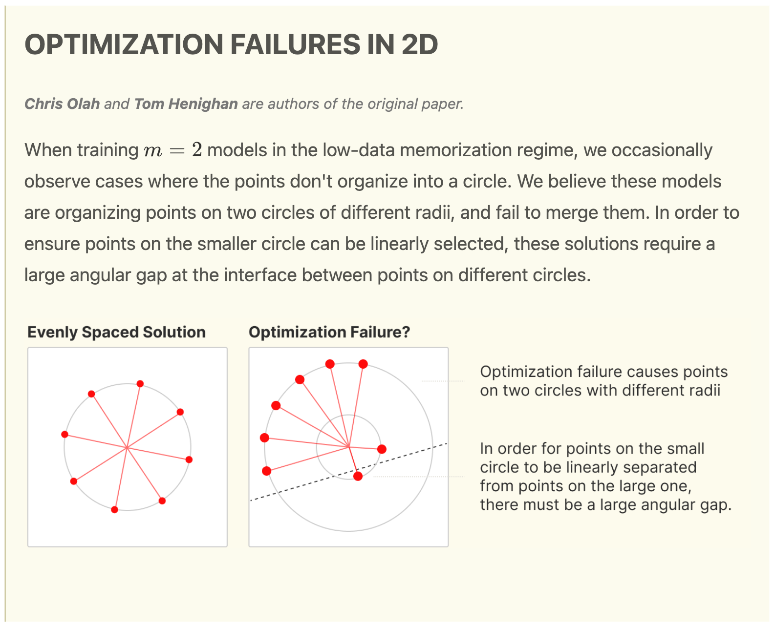
- A best-effort implementation will have to equalize the columns of $A$, which necessarily assumes that hidden features of the $\text{ReLU}$ model we’re trying to extract are equal magnitude, which is completely false. Recall the “Optimization Failure” phenomenon where features with identical statistical properties in the dataset ended up having different feature magnitudes:
![Anthropic Optimization Failure post]()
- ICA will run into problems trying to extract features that have non-zero correlation with each other, such as pairs of hierarchical features (e.g. “Fish” and “Salmon”).
In general, I get the feeling that feature extraction is much more like a classic compressed sensing problem than would initially seem. It is especially so if we were to focus on embeddings in only the residual stream of language models, because the residual stream is subject to only linear operations. I.E. it seems very plausible that Transformer blocks are doing CRUD operations on features, while the residual stream is simply a memory bank that contains a linear superposition of features. If so, given how established compressed sensing is as a problem and how much work has been done on it, I think it is much more worthwhile to trace through the discourse of correlated overcomplete feature extraction and derive a better method from there, or if not, at least a satisfying argument of why this problem of feature extraction is “too hard.”