
Principle Component Analysis (PCA) is a fundamental dimension-reduction technique that we all know to identify the top $k$ components of a set of $d-$ dimensional data points, where $k < d$. In particular, the top principle components of the data are simply the directions in the data subspace along which the data set has the highest variance. However, there is a very elegant extension of PCA that allows us to use this information to actually characterize different groups of data that have difference covariances and even perform classification on them. This transformation is the Common Spatial Pattern algorithm. It’s extremely elegant, and has extremely effective uses that are not well known, chiefly in areas like finance and neuroscience.
Contents
- PCA
- CSP Derivation
- Applications
1. PCA
Suppose you have a dataset $X \in \R^{N \times d}$; to keep things simple, we’ll assume $d = 2$, and $N$ is some large number, like $500$. Suppose further that your data is inconveniently rotated, like this:
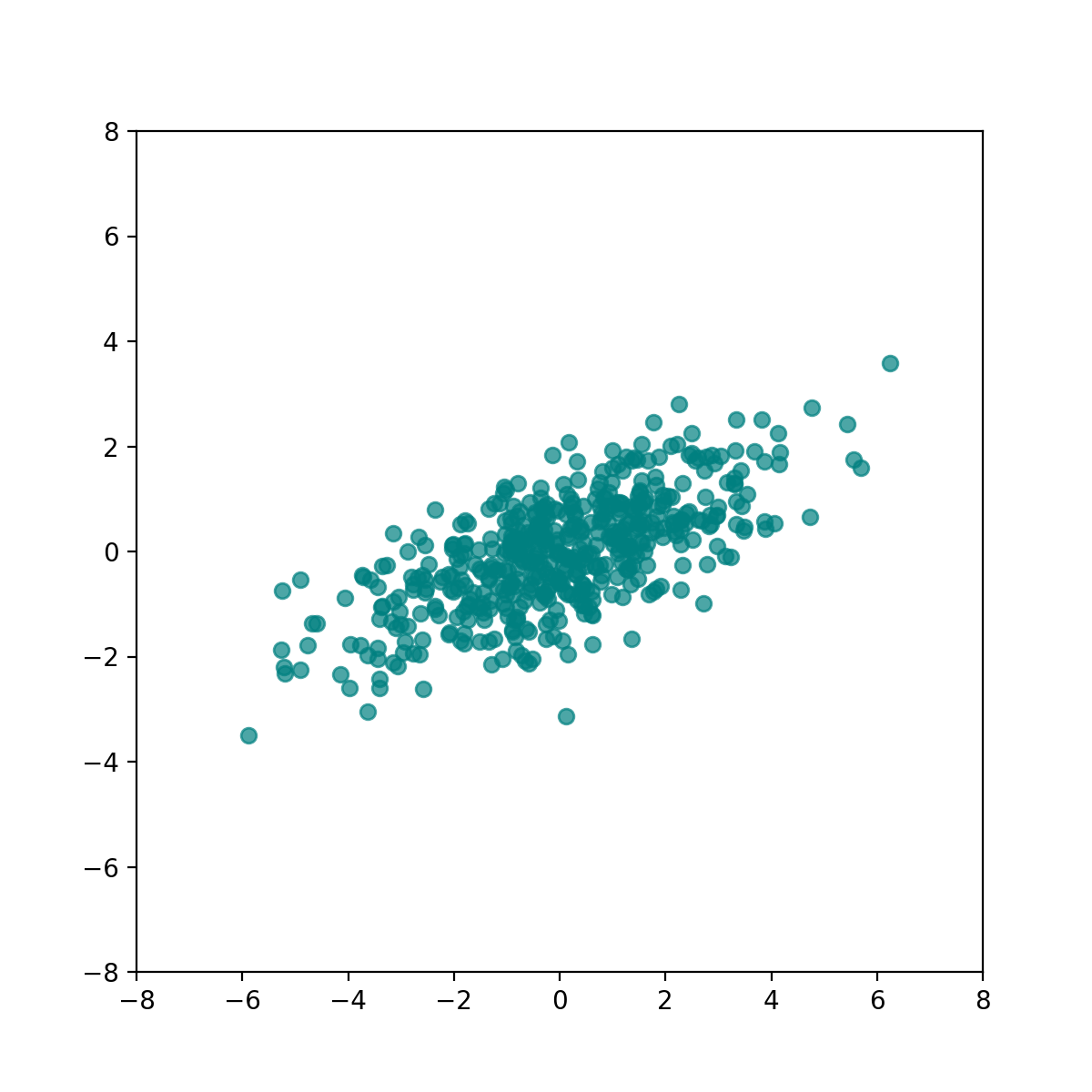
Why would someone describe this as inconveniently rotated? Suppose you were a school teacher and wanted to figure out in which subjects your students were scoring the widest range of scores (most unpredictable / inconsistent performance). If you had your dataset of student scores $X$ such that the columns of $X$ were the student scores for a certain subject, then doing this would be really easy - all you have to do is muse to yourself that the columns of your data (subjects) already represent the directions along which you want to measure variance, and take the column-wise variance of $X$, and see which column produced the greatest column-wise variance. Done!
In reality, it can be exceedingly hard to know what directions are important to us. For example, it may be intuitive to think that, if you were running a real estate company renting apartments, the important axes would be square footage, number of bedrooms, and the reciprocal of distance to the nearest train station. However, the real predictors of price may not at all nicely be one, or an equal combination of any of those quantities. It may be some unequal combination of square footage and number of bedrooms, for example. If the first column of $X$ is square footage and the second column of $X$ is number of bedrooms, a simple but inconvenient true predictor of price could be a combination of square footage and number of bedrooms in 80% - 20% ratio. This means that the market equilibrium would be such that apartments tend to increase square footage four times as fast as number of bedrooms. The above plot would illustrate such a dataset of apartment configurations, where the horizontal-axis is square footage, and the vertical-axis is number of bedrooms. A pertinent question to ask, analogously to the above test scores scenario, is how valuable an apartment is, given this slanted axis of value.
In math, the goal is very simply to rotate the data such that the axes of greatest variance become the normal basis vectors $e_1, e_2, …$. This is very briefly done by taking the eigendecomposition of $X$:
\[\begin{align*} X & = Q \Lambda Q^{-1} \end{align*}\]Remember that every matrix (I’m talking specifically about $X$ here), can be thought of as a rotation ($Q^\top$), followed by a stretch ($\Lambda$), followed by another rotation ($Q$). There’s more formal intuition that can be gleaned from this, but it suffices to reason that because the stretch $\Lambda$ is in the eigenbasis of $X$, $Q$ can be thought of as a rotation from the eigenbasis of $X$ to the normal basis ${e_1, e_2, …}$. So, to rotate $X$ into the normal basis, we just do $XQ$: 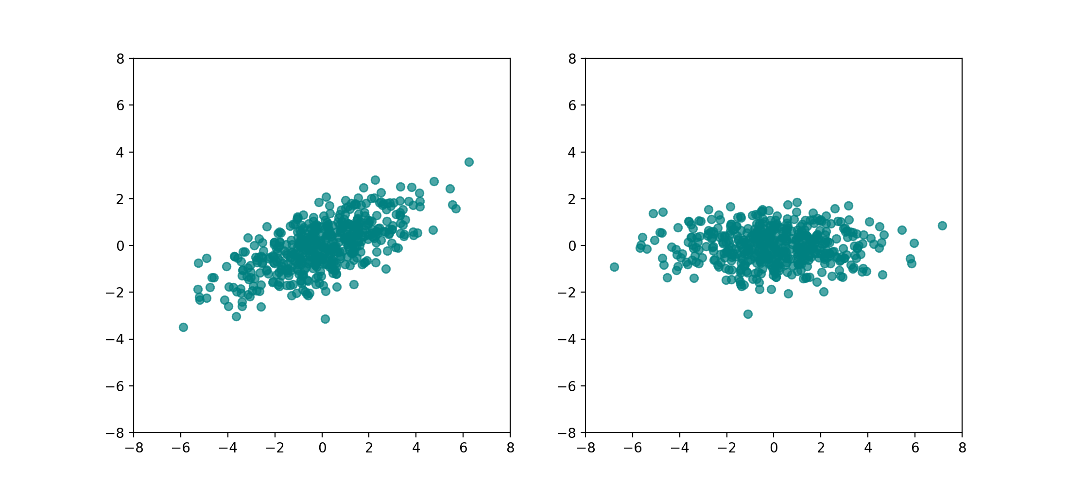
2. CSP
So we know that PCA rotates data, in a way identifying the principle components (axes) along which the variance of the data is the greatest. Suppose we had two data classes / datasets $X_1, X_2$ instead, e.g. a dataset of apartment configurations in California, and another in London. Suppose even further that these data have been mean normalized (such that they are centered at the origin).
It may not be so natural in this example, but a lot of real data in the world come from sources that are not shift-invariant, so a crucial preprocessing step is to normalize by the mean. An example would be the brain - baseline levels of activity can change drastically from day to day, even in the same person.
This means that our datasets overlap like this:
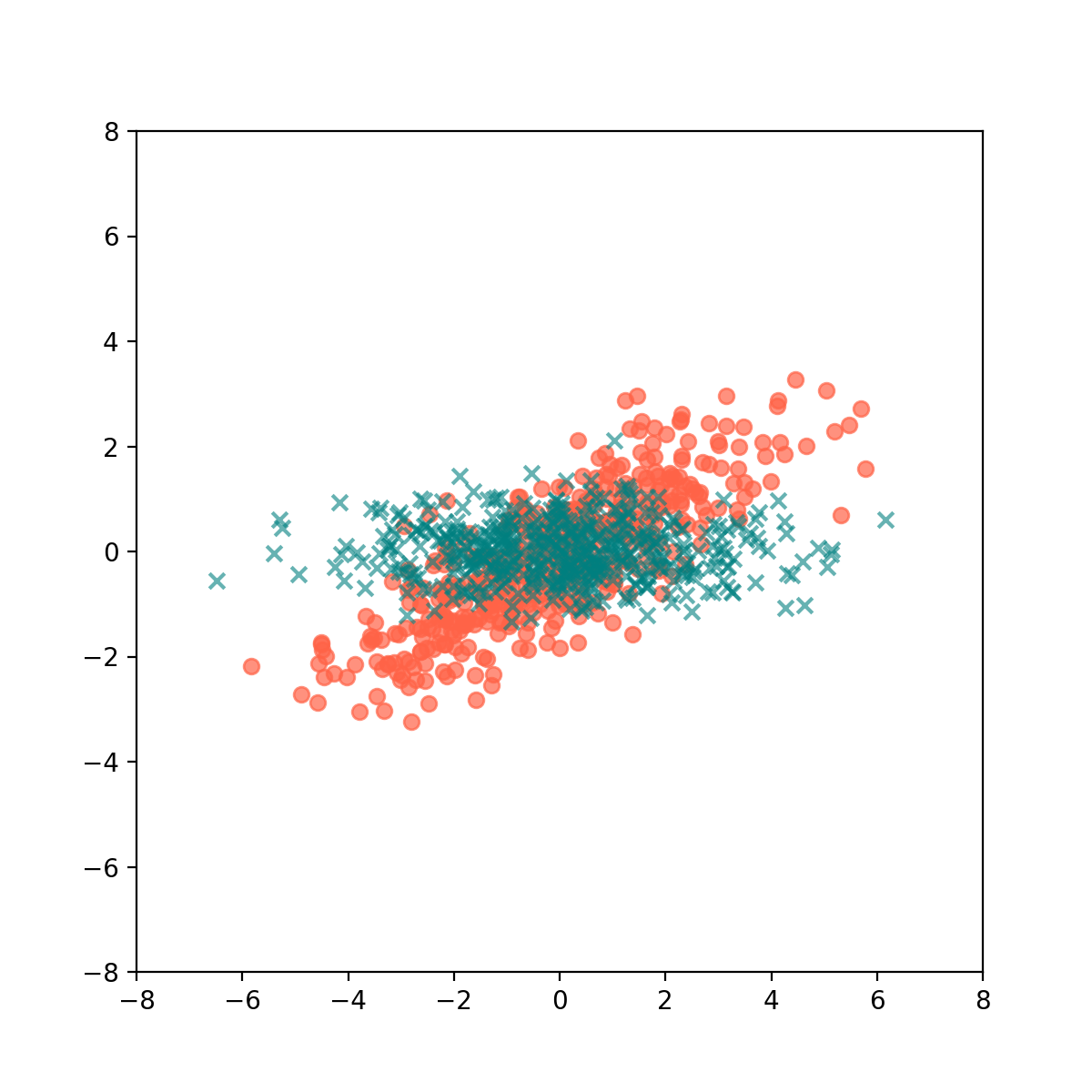
Our goal is to be able to rotate the data in such a way that these two Gaussian blobs look as different as they possibly could to each other. A pretty evocative and intuitive phrase one could use to describe this is to orthogonalize their variances.
In math, we are assuming that there is some shared eigenspace (which there will be, if the two datasets exist in the same subspace) between the covariance matrices of the two datasets, and we want to find a rotation into that shared eigenspace. The more proper terms for this, is the simultaneous diagonalization of the 2 covariance matrices.
\[\begin{align*} \text{Cov}(X_1) & = \frac{1}{N_1}X_1X_1^\top, \\ \text{Cov}(X_2) & = \frac{1}{N_2} X_2 X_2^\top, \\ \text{Cov}(X_2)^{-1} \text{Cov}(X_1) & = Q \Lambda Q^\top \end{align*}\]Once you’ve gotten $Q$, we can likewise apply $Q$ to $X_1$ and $X_2$:
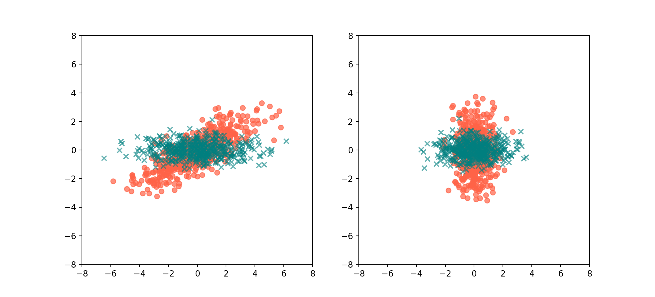
This is useful because, if someone were to throw you a dataset and get you to figure out if it was more likely from the California apartment market or the London one, you can simply apply the rotation $Q$, and take the column-wise variance of the the rotated data. If the vertical variance is much larger than the horizontal variance, then it likely belongs to California, otherwise it’s London.
3. Application: EEG Motor Imagery
All this talk of apartments may not seem super relevant, so perhaps it’ll feel more motivating if I were to give an actual useful example: Motor Imagery (MI). MI is a mental process by which humans mentally rehearse or simulate a given action, e.g., imagining waving one’s hand or picking up an object, without performing the actual motor movements. This can be useful in constructing Brain-Computer Interface applications for people who have lost motor abilities in their limbs.
The problem set up is this: suppose a person were wearing an Electroencephalogram (EEG) net / cap, which is basically an array of sensors (called “channels”) that each pick up on the local electrical activity surrounding it coming from the brain, and imagining 2 possible actions - squeezing a stress ball with their left hand, or squeezing a stress ball with their right hand. Given some training data in the form of a few 5-second-long multi-channel EEG time-series per action, can we fit a model that allows us to classify future unseen EEG data?
Turns out, CSP works super well for this, which is quite appalling given how ostensibly complex the brain’s electrical signals are. The intuition is that neurons in different areas of your brain will fire at different intensities when evoking MI in your left hand versus in your right hand. In mathematical terms, the different channels of the EEG time-series data covary with each other in a different way for different imagined actions, i.e. they have different covariance matrices! Applying the CSP rotation to this, and then fitting a simple linear discriminator on the variances of such time-series data allows a classification accuracy of naer 90%, which sounds absolutely incredible to me.