
Linear Regression (LR) is hands-down THE most useful and ubiquitous tool in statistics. Everything derives from linear regression; even the most complex statistical models at some point have to be reasoned or tested in terms relevant to LR. This is part of what makes the fundamentals of statistics so simple, yet profound. In this post, we will briefly derive and intuit several basic facts about the Ordinary-Least-Squares (OLS) predictor coefficients, $\hat{\beta}$, that I have found myself returning to reference all the time.
Contents
- Terminology
- Deriving beta-hat: $\hat{\beta}$
- Mean of beta-hat: $\mathbb{E}[\hat{\beta}]$
- Covariance of beta-hat: $\text{Cov}(\hat{\beta})$ $\newcommand{\betahat}{\hat{\beta}}$ $\newcommand{\E}{\mathbb{E}}$ $\newcommand{\Cov}{\text{Cov}}$ $\newcommand{\mleft}{\left[ \begin{matrix}}$ $\newcommand{\mright}{\end{matrix} \right]}$ $\renewcommand{\R}{\mathbb{R}}$ $\newcommand{\eps}{\varepsilon}$ $\newcommand{\ltwo}[1]{ \lVert #1 \rVert_2}$ $\renewcommand{\argmin}{\text{argmin}}$
1. Terminology
First, we recap terminology that is standard in the world of statistics. In a standard LR problem, we need to have:
$X \in \R^{n \times p}$: The “Design Matrix”
\[X = \mleft \vert & \vert & & \vert \\ \mathbf{1} & X_1 & \cdots & X_{p-1} \\ \vert & \vert & & \vert \mright\]A matrix of $n$ data points, where each data point has $p$ “predictors” or “covariates,” inclusive of the $1$’s that you have to concatenate to all the data so that the offset ($y$-intercept) can be calculated as part of the regression. This means that you have $n$ data points, each of them having $p - 1$ features, such that the design matrix can be an $n \times p$ matrix.
$y \in \R^n$: The “Response” or “Target”
\[y = \mleft y_1 \\ \vdots \\ y_n \mright\]This is simply the dependent variable. E.g., if we are trying to perform LR on real-estate features like number of bedrooms and square footage to price, then a single row of $X$ corresponds to said features, while the corresponding row of $y$ corresponds to the price of the house associated with said features.
2. Deriving $\betahat$
The standard linear model is rather intuitive. Given some features $X$, we believe that these features map on rather “fuzzily” to a target $y$:
\[y = X\beta + \eps\]where $\eps$ is an independent noise variable, about whose distribution we know nothing beyond the mean ($0$) and variance ($\sigma^2$):
\[\eps \sim (0, \sigma^2)\]Note that this is just an assumed model. The assumption is that there is some “true” $\beta$ that generates the targets $y$ given some set of features $X$. We don’t know this “true” $\beta$, so our goal is find an estimate of $\beta$, which is usually denoted by $\betahat$, that allows us to predict the targets with as little error as possible. There are many measures of such “error,” but the measure of choice is the sum of the squares of the differences between the targets ($y$) and our predictions ($\hat{y}$), also known as the “residual sum of squares” (RSS):
\[\begin{align*} \betahat & = \argmin_\beta \ltwo{y - \hat{y}}^2 \\ & = \argmin_{\beta} \ltwo{y - X\beta}^2 \end{align*}\]2.1 Why L2-norm?
There are two main reasons we use the L2-norm of $(y - \hat{y})$ as the desired measure of error.
- The first is that taking the derivative of the L2-norm is much easier than doing that for, say, L1-norms. This is mainly a historical reason that has its roots in the times when humanity didn’t have computers.
- The second is that the OLS Coefficients can be shown to be the Best Linear Unbiased Estimator (BLUE), which is the famous Gauss Markov Theorem.
2.2 Deriving $\betahat$ with just Calculus
This is not my preferred way of doing it, but it’s really fast and easy. To find the $\beta$ that minimizes $\ltwo{y - X\beta}^2$, we simply take the derivative of this and set it to $0$:
\[\begin{align*} \nabla_{\beta} \left( 2 (y - X\beta)^\top(y - X \beta)\right) & = \nabla_\beta \left( y^\top y - y X \beta - \beta^\top X^\top y + \beta^\top X^\top X \beta \right) \\ & = \nabla_\beta \left( -2 \beta^\top X^\top y + \beta^\top X^\top X \beta \right) \\ & = - 2 X^\top y + 2 X^\top X \beta \end{align*}\]Set the above to $0$:
\[\begin{align*} - 2 X^\top y + 2 X^\top X \betahat & = 0 \\ X^\top X\betahat & = X^\top y \text{ (} \unicode{x201C} \text{Normal Equation")} \\ \betahat & = (X^\top X)^{-1} y \end{align*}\]Notice that in the second last step, we derived what is sometimes called the “Normal Equation” for OLS LR.
2.3 Deriving $\betahat$ with Geometry
This derivation has very strong intuition behind it but requires us to visualize the geometry of the error minimization. We shall work through an example of $n = 3$ data points, each with only $(p-1) = 1$ feature, for a total of $p = 2$ features (inclusive of the $1$ for the intercept). This is the only subspace that we can graph out in 3D space.
We first note that the quantity we are minimizing is simply the square of the L2-norm of the difference between 2 vectors:
\[\ltwo{y - \hat{y}}^2\]$\hat{y}$ must be $\in \mathcal{R}(X)$.
In particular, $\hat{y}$ and $y$ are both $\in \R^3$. A key requirement of LR is that we want to be able to express our predictions $\hat{y}$ as a linear combination of our features $X_1, \cdots, X_p$, where $X_i$ denotes the $i$-th column of $X$. That is, we require our predictions to have the form $\hat{y} = X\betahat$. This means that $\hat{y}$ is necessarily in the column-space (“Range,” denoted by $\mathcal{R}$) of $X$.
To give an example, if our design matrix looks like this:
\[X = \mleft 1 & 2 \\ 1 & 3 \\ 1 & 4 \mright\]Then $\mathcal{R}(X)$ is simply the span of the vectors:
\(X_1 = \mleft 1 \\ 1 \\ 1 \mright, X_2 = \mleft 2 \\ 3 \\ 4 \mright\).
This is a $(p=2)$-dimensional plane in $\R^{n = 3}$:
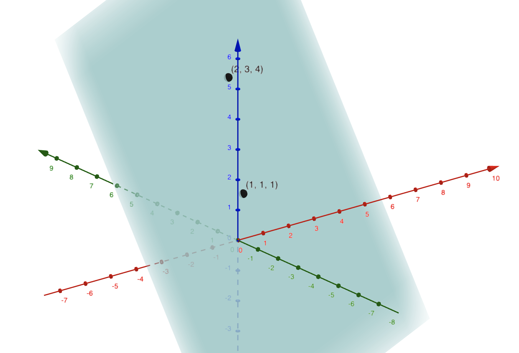
Somewhere on this plane lies an ideal $\hat{y}$ that has minimal L2-distance from $y$.
Note that $y$ need not be on this plane, and as long as there is some noise ($\eps$), $y$ is almost certainly never on this plane.
The ideal $\hat{y}$ is therefore simply the projection vector of $y$ onto this plane. This means that $\hat{y} = Hy$, where $H$ is the projection matrix (also called the “Hat matrix”, because it puts a hat on $y$) that projects $y$ onto $\mathcal{R}(X)$. There is a rather standard form of such a projection matrix:
\[H = X(X^\top X)^{-1} X^\top\]If we plug this back into $\hat{y} = Hy$, we have:
\[\begin{align*} \hat{y} & = X(X^\top X)^{-1} X^\top y \\ & = X \betahat \\ \Rightarrow \betahat & = (X^\top X)^{-1} X^\top y \end{align*}\]Done! Clean and simple! This idea generalizes to any number of data points $n$ and predictors $p$, so long as $n \geq p$, which should be true, since LR is about trying to draw out a relationship to a small number of high-signal predictors from a pile of data.
If $n \ngeq p$, then $(X^\top X)$ will not have an inverse since it’s not full-rank. There are instances where we still have to work with LR in such a scenario, so other variants of LR like Ridge Regression are used instead.
It’s just that with a greater number $n$ of points, the $\R^n$ space is no longer visualizable, and with a greater number $p$ of predictors, so too becomes the $p$-dimensional subspace. But the intuition does indeed generalize!
3. Distribution of $\betahat$
Because $\betahat$ is a fitted set of parameters that depends on the observed data $X$ and $y$, $\betahat$ itself is a random variable that follows a random distribution. If we know the distribution of $\betahat$, we can reason about what the expectation of $\betahat$ is, and how much uncertainty our guess of the true $\beta$ has.
3.1. Expectation of $\betahat$: $\E[\betahat]$
The punchline intuition is this: if you had a sample of data, from which you derived a $\betahat$, what reason would you have to believe that the true $\beta$ is different from this $\betahat$? If your sample is at all representative of the true population, which we have to assume it is, then you would also expect that your $\betahat$ is actually the true $\beta$.
Mathematical Proof:
\[\begin{align*} \betahat& = (X^\top X)^{-1} X^\top y \\ & = (X^\top X)^{-1} X^\top (X\beta + \eps) \\ & = \beta + (X^\top X)^{-1} X^\top \eps\\ \E[{\betahat}] & = \E[\beta] + \E[(X^\top X)^{-1}X^\top \eps] \\ & = \beta + \E[(X^\top X)^{-1} X^\top] \E[\eps] \text{ (because } \eps \perp X \text{)} \\ & = \beta + \E[(X^\top X)^{-1} X^\top] \cdot 0 \\ & = \beta \end{align*}\]3.2. Covariance of $\betahat$: $\Cov(\betahat)$
The covariance of $\betahat$ is harder to derive, and requires some linear-algebraic tricks. But nonetheless, it’s an important proof, and the proof below, in particular, is what I believe to be the easiest proof.
\[\begin{align*} \Cov(\betahat) & = \Cov[\beta + (X^\top X)^{-1} X^\top \eps] \\ & = \Cov[\beta] + \Cov[(X^\top X)^{-1} X^\top \eps] \\ & = 0 + \left((X^\top X)^{-1} X^\top\right) \Cov(\eps)\left((X^\top X)^{-1} X^\top \right)^\top\text{ (fact: } \Cov(Ax) = A \Cov(x) A^\top \text{)} \\ & = \left((X^\top X)^{-1} X^\top\right) \sigma^2 \mathbf{I} \left((X^\top X)^{-1} X^\top \right)^\top \\ & = \sigma^2 \mathbf{I} \left((X^\top X)^{-1} X^\top\right) \left((X^\top X)^{-1} X^\top \right)^\top \text{ (can move } \sigma^2 \mathbf{I} \text{ out because it's diagonal)} \\ & = \sigma^2 (X^\top X)^{-1} X^\top X (X^\top X)^{-1} \text{ (because } (X^\top X) \text{ is symmetric, as is } (X^\top X)^{-1} \text{)} \\ & = \sigma^2 (X^\top X)^{-1} \end{align*}\]