The Gaussian (Normal) Distribution can be found everywhere; it is also a laughably common tendency for statisticians and engineers to describe any stochastic phenomenon using Gaussians. Though we can easily recognize it for its distinctive bell-curve shape, its formula is much less palatable. There’s even a $\pi$ in there, the reason it’s there being not at all obvious:
\[f_{\mathcal{N}(\mu, \sigma^2)}(x) = \frac{1}{\sqrt{2 \pi} \sigma} \exp \left(-\frac{1}{2} \left( \frac{x - \mu}{\sigma}\right)\right)\]I think there’s a certain “universality” of the Gaussian Distribution because of how it can be traced back to the Binomial Distribution, which is in turn somewhat universal because there always exists a way to break down a stochastic problem into a series of “yes / no” questions. Here are some examples of what I mean:
- Test scores that resemble Gaussians (e.g. a score out of 100) can be broken down into a series of 100 binary (“yes / no”) problems, wherein the total score is simply how many of these 100 sub-problems resulted in a coin-flipped “yes”.
- A human adult’s height could be lower-bounded at, say, 50 cm (about 1.7 feet) and upper-bounded at about 250 cm (about 8.2 feet), with each cm of height above 50 cm being thought of as a “yes / no” problem (up to 250 cm), such that the height of any random given person is simply 50 cm + the number of coin-flipped “yes”-es in additional cm.
Of course, binomial problems are inherently bounded; unlikely the Poisson Distribution, for example, the range of values one can expect in a binomial problem does not go up to infinity. Indeed, for this reason, some may disprefer thinking of Gaussians as coming from Binomial Distributions - that is valid, but shall remain outside the scope of this post. In this post, we shall demonstrate the approximation of the Binomial Distribution to the Gaussian Distribution, and even derive the Gaussian PDF from the Binomial PDF.
\[\newcommand{\Normal}{\mathcal{N}}\]Contents
- The Central Limit Theorem
- Gauss’ Integral
1. The Central Limit Theorem & Pascal’s Triangle
The Central Limit Theorem simply states that as you draw a larger and larger number of samples, your distribution of observed values converges to the Gaussian Distribution. One way of writing that is this:
\[\sqrt{n}(\overline{X} - \mu) \to \Normal(0, \sigma^2)\]but I really prefer this way of writing it:
\[\begin{align*} \overline{X} & \to \Normal \left(\mu, \frac{\sigma^2}{n} \right) \\ \Rightarrow \sum_{i=1}^n X_i & \to \Normal \left(n \mu, n\sigma^2 \right) \end{align*}\]A really impactful way of verifying this for ourselves is to illustrate the approximation of a binomial problem to a Gaussian Distribution
1.1. Coin Flips
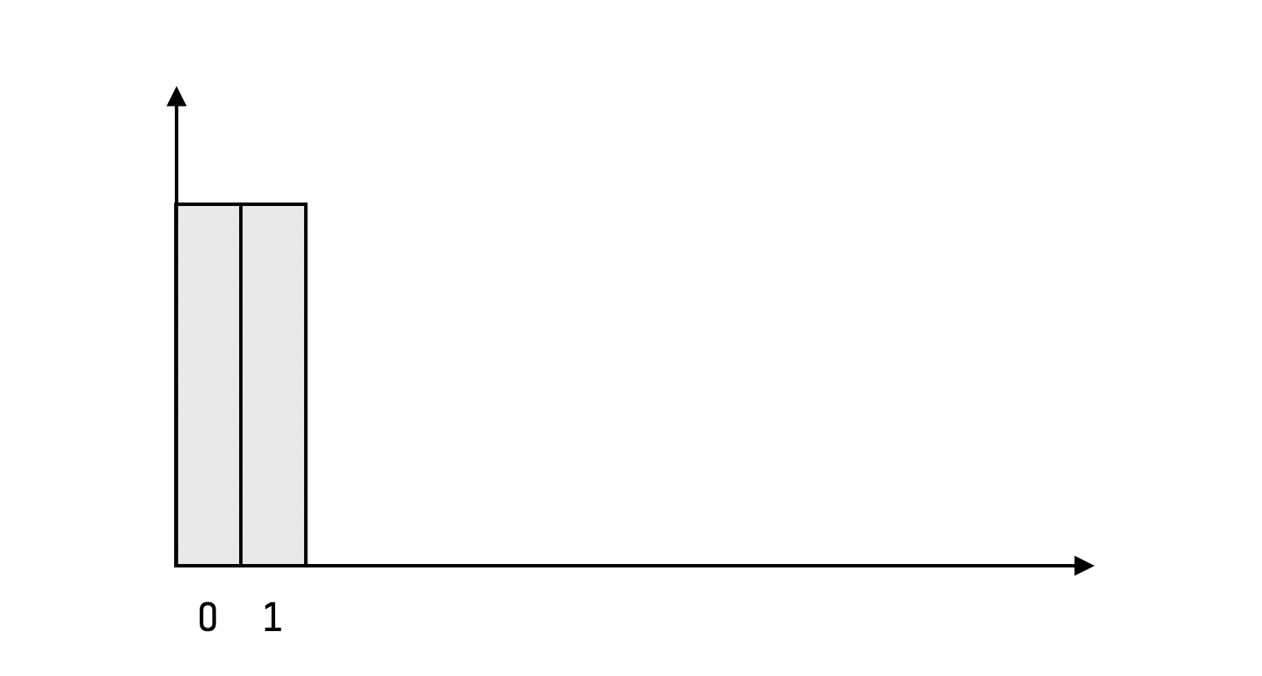
Consider the problem of flipping a fair coin. Each of heads and tails have an equal chance of coming up. Each time heads comes up, you gain a point in rewa; nothing gained or lost when tails comes up. What’s the distribution of total reward for 1 toss? It’s simply 50% chance for 0 reward, and 50% chance for 1 point. The probability mass function (PMF) looks like this (horizontal axis: total reward, vertical axis: probability):
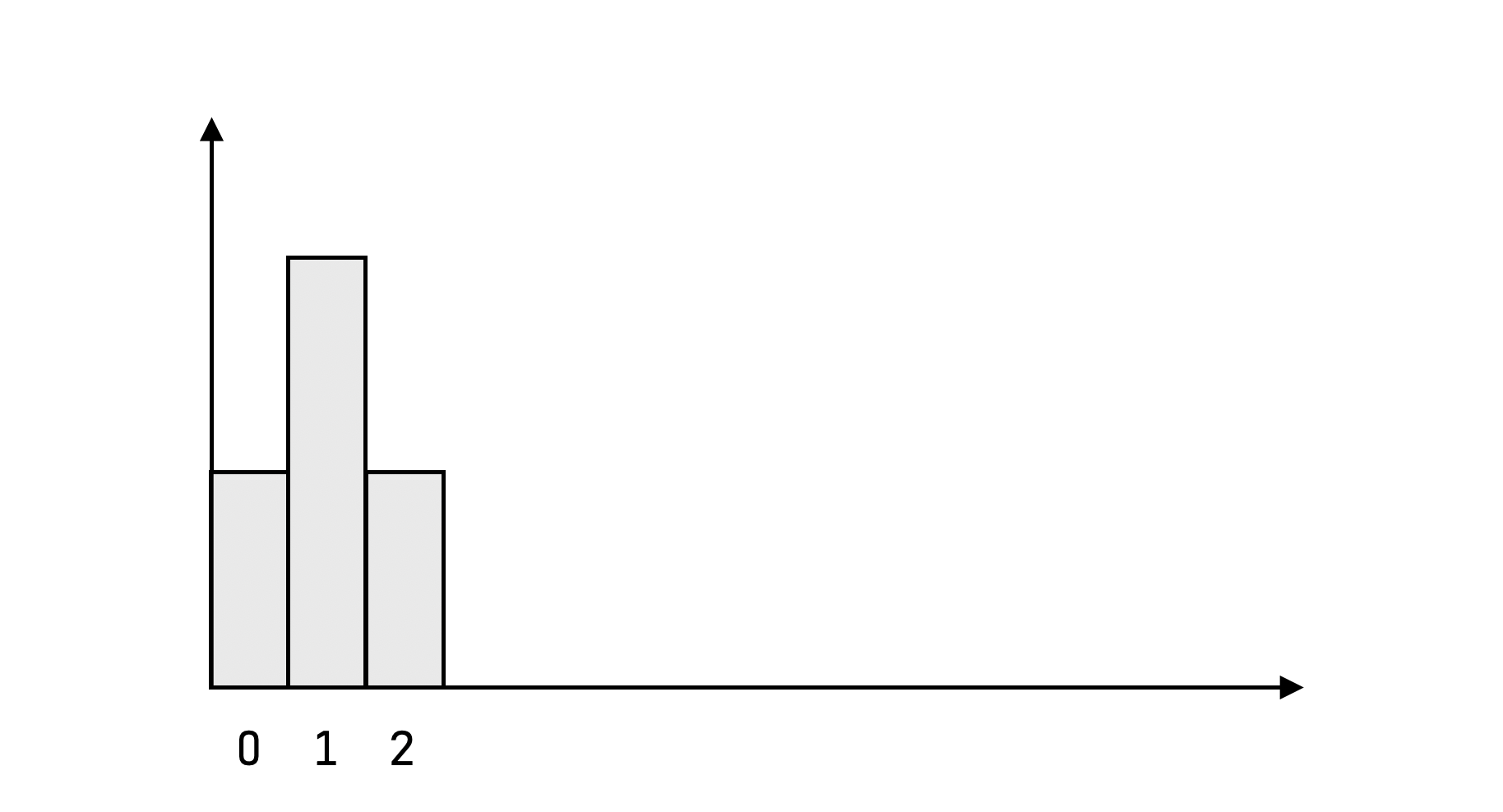
Suppose you flipped twice, what does the distribution look like now? There was only one way to get 0 points, and one way to get 2 points, but two ways to get 1 point (two ways of choosing which coin lands on heads and hence which coin lands on tails).
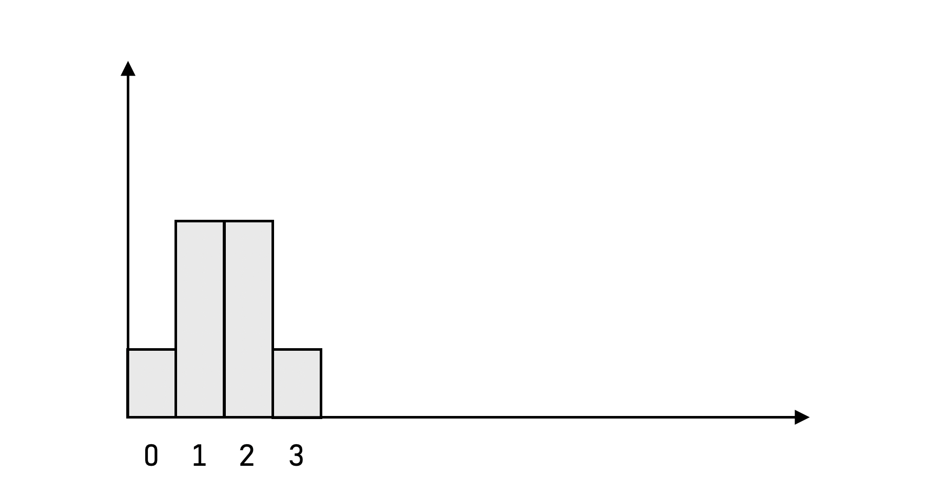
What about three flips? You’ve got:
- $\binom{3}{0} = 1$ way to choose $0$ coins to land on heads.
- $\binom{3}{1} = 3$ ways to choose $1$ coin to land on heads.
- $\binom{3}{2} = 3$ ways to choose $2$ coins to land on heads.
- $\binom{3}{3} = 1$ ways to choose all $3$ coins to land on heads.
1.2. Pascal’s Triangle
Here’s an illustration of the PMFs of total reward for up to 6 tosses:
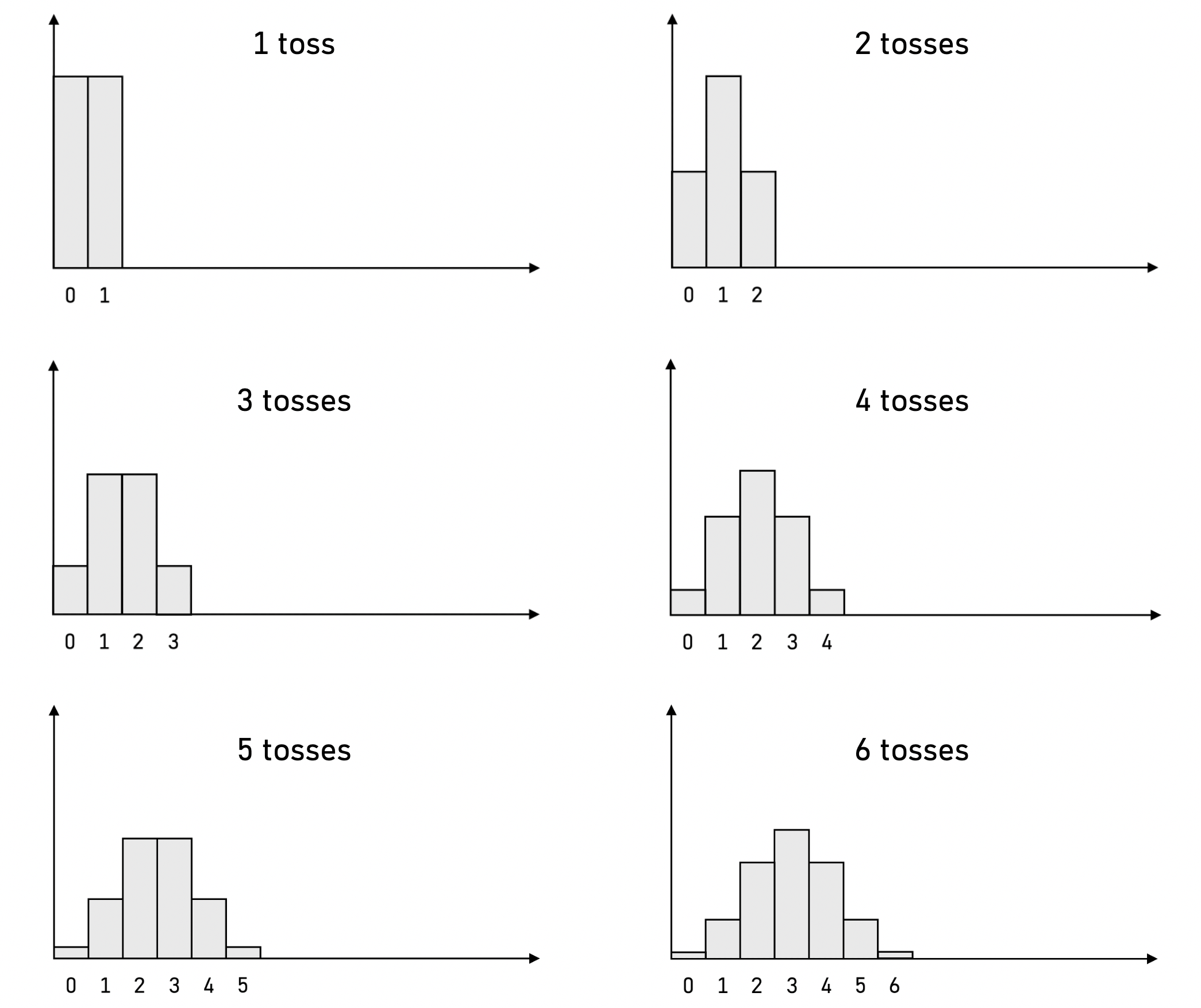
You can observe that the PMFs already start to look more and more like the distinctive Gaussian curve. The shapes of these PMFs are governed entirely by the Pascal’s Triangle, since the Pascal’s Triangle tells us all the binomial coefficients, a.k.a. how many ways there are to choose a subset of size $k$ (i.e. coins that land on heads) from a set of $n$ elements (i.e. total flips):
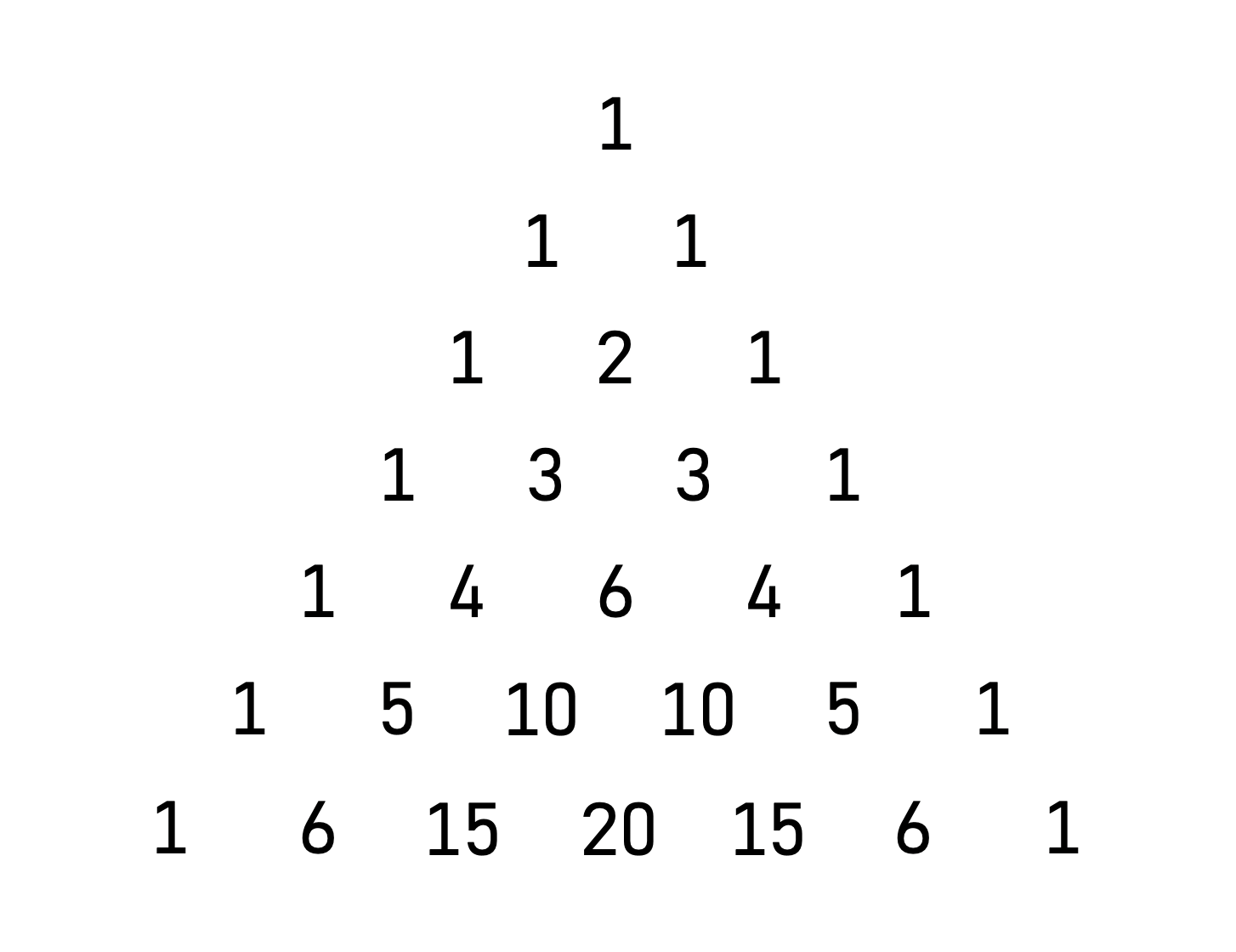
In fact, since the shapes of these PMFs are entirely dependent on the Pascal’s Triangle, we can simply use the formula for the binomial coefficients to analytically derive the PMF of total reward over $n$ flips! There are only two things to note here. Firstly, we recall the binomial coefficient formula:
\[\binom{n}{k} = \frac{n!}{k!(n-k)!}\]Secondly, we note that the probability of all the events must sum to $1$ for this to be a valid PMF. Therefore, all the binomial coefficients must be normalized by the total number of ways to choose any number of elements from a universe containing $n$ elements (i.e. the cardinality of the entire space of events). This is simply the size of the superset of $n$ elements, which is simply $2^n$.
1.3. Stirling’s Approximation
Thus far, we have already conceptually derived the Gaussian-ization of the binomial distribution. If we simply combined the above two points and wrote out the PMF, we have:
\[f(X = x) = \frac{n!}{x!(n-x)! \times 2^n}\]From here, we have two problems:
- We need to make this amenable to continuous domains, as Gaussians are. The above PMF is fine for discrete domains ($X$) but not quite for continuous ones.
- There is an upper limit imposed by our binomial approximation, as given by $n$. From a binomial context, if we only tossed a coin $n$ times, there can only be $n$ heads at most. In a Gaussian distribution, there is no such upper limit. A similar problem exists for the lower limit.
The first problem is much more solvable than the second. In particular, we may either use the generalization of the factorial (i.e. the Gamma Function, $\Gamma$) or Stirling’s approximation. We will use Stirling’s approximation because:
- The Gamma Function has non-obvious properties that are completely non-trivial to derive, such as $\Gamma(1/2) = \pi$.
- Stirling’s approximation allows us to partially address the second problem as well.
So, having understood the motivation behind Stirling’s Approximation, we finally state it:
\[n! \approx \sqrt{2 \pi n} \left( \frac{n}{e} \right)^n\]So, plugging it into the above PMF equation, we have:
\[f(X = x) = \frac{\sqrt{2 \pi n} \left( \frac{n}{e} \right)^n}{ \sqrt{2 \pi x} \left( \frac{x}{e} \right)^x \sqrt{2 \pi (n - x)} \left( \frac{n - x}{e} \right)^{n-x} \times 2^n }\]We now use some intuition from having seen the shape of these PMFs. In particular, we remember that these PMFs are symmetric about the mean of $\mu = n/2$. Perhaps then, we can wrangle with the above formula by expressing it in terms of $\mu$:
\[\begin{align*} f(X = x) & = \sqrt{\frac{n}{2\pi x(n - x)}} \times \frac{\left( \frac{n}{e} \right)^n}{ \left( \frac{x}{e} \right)^x \left( \frac{n - x}{e}\right)^{n-x} \times 2^n} \\ & = \sqrt{\frac{n}{2\pi x(n - x)}} \times \frac{n^n}{x^x (n - x)^{n-x} \times 2^n} \\ & = \sqrt{\frac{n}{2\pi x(n - x)}} \times \left( \frac{n}{2} \right)^n \left( \frac{1}{x^x (n - x)^{n - x}} \right) \\ & = \sqrt{\frac{n}{2\pi x(n - x)}} \times \mu^n \left( \frac{1}{x^x (n - x)^{n - x}} \right) \\ & = \sqrt{\frac{n}{2\pi }} \times \mu^n \left( \frac{1}{x^{x + 1/2} (n - x)^{n - x + 1/2}} \right) \\ & = \sqrt{\frac{4 \sigma}{2\pi \mu }} \times \mu^{n+1} \left( \frac{1}{x^{x + 1/2} (n - x)^{n - x + 1/2}} \right) \\ & = \sqrt{\frac{1}{\pi}} \times \left( \frac{\mu}{x} \right)^{x + 1/2} \left( \frac{\mu}{n - x} \right)^{n - x + 1/2} \end{align*}\]From here on: writing in progress
Note that:
\[\begin{align*} \sigma & = np(1 - p) = \frac{n}{4} \\ \mu & = np = \frac{n}{2} \\ \therefore \sigma & = \frac{\mu}{2} \end{align*}\]1.3.1 Maclaurin’s Series
\[\begin{align*} \ \end{align*}\]Old calculation
\[\begin{align*} f(X = x) & = \frac{\sqrt{2 \pi n} \left( \frac{2\mu}{e} \right)^{2\mu}}{ \sqrt{2 \pi x} \left( \frac{x}{e} \right)^x \sqrt{2 \pi (2\mu - x)} \left( \frac{2\mu - x}{e} \right)^{2\mu-x} } \\ & = \frac{\sqrt{2 \pi n} \left( \frac{2\mu}{e} \right)^{2\mu}}{ \sqrt{2 \pi (\mu - (\mu - x))} \left( \frac{\mu - (\mu - x)}{e} \right)^{\mu - (\mu - x)} \sqrt{2 \pi (\mu + (\mu - x))} \left( \frac{\mu + (\mu - x)}{e} \right)^{\mu + (\mu-x)} } \\ & = \frac{\sqrt{n} \left( \frac{2\mu}{e} \right)^{2\mu} }{\sqrt{2 \pi} \times \sqrt{(\mu - (\mu - x))(\mu + (\mu - x))} \left( \frac{\mu - (\mu - x)}{e} \right)^{\mu - (\mu - x)} \left( \frac{\mu + (\mu - x)}{e} \right)^{\mu + (\mu-x)} } \\ & = \frac{\sqrt{n} \left( \frac{2\mu}{e} \right)^{2\mu} }{\sqrt{2 \pi} \times \sqrt{(\mu^2 - (\mu - x)^2} \left(\frac{1}{e}\right)^{2\mu} \left(\mu^2 - (\mu - x)^2 \right)^{\mu - (\mu - x)} \left( \mu + (\mu - x) \right)^{2(\mu-x)} } \end{align*}\]Scratch
\[\begin{align*} x(n - x) & = (\mu - (\mu - x))(\mu + (\mu - x)) \\ & = \mu^2 - (\mu - x)^2 \\ & = 2\mu x - x^2 \end{align*}\]