T-test: Motivation, Definition, and Derivation

Contents

1. Contextual Problem.
2. Defining $s^2$, a.k.a the sample variance ($\sigma^2$).
3. Motivating the $T$ test.
4. Deriving the $T$ statistic.

1. Contextual Problem

A key objective of analysis of large systems across many domains is to see if the quantifiable metrics of the large system do indeed adhere to one’s expectations. For example, you are running a flour packaging factory and want to see if the mass of each pack of flour indeed has some expected value. Or perhaps you are given a sample of flour pack masses that somebody has measured and want to see if that sample of flour packs indeed came from your factory. Whatever it is, you would typically sample a bunch of observations (measure a bunch of flour packs in this case), compute sample statistics (sample mean $\overline{X}$ and variance $\frac{1}{n} \sum(X_i - \overline{X_n})^2$), and try to make comments about how different these look from the expected (“assumed”) distribution statistics (population mean $\mu$ and variance $\sigma^2$). The tests that are typically done with these statistics are the $Z$ test and the $T$ test. The former is significantly easier to understand, but the latter really takes after the former, so we’ll start with the $Z$ test and use our intuition of that to reverse-engineer the $T$ test, as it was actually done during its invention.

2. Defining $s^2$, the unbiased estimator of $\sigma^2$

Let’s define some terms. Given a sample of $n$ observations $X_1, \cdots, X_n$, this is the sample mean:

\[\begin{equation*} \overline{X_n} = \frac{1}{n}\sum_{i=1}^n X_i \end{equation*}\]

Which is markedly different from the true population mean $\mu$. “Population” refers to the universe of all instances of the things you’re trying to measure. This is the sample variance:

\[\begin{equation*} \frac{1}{n}\sum_{i=1}^n\left(X_i - \overline{X_n} \right)^2 \end{equation*}\]

Notice that I did not assign it any symbol. This is because we’ll be working with the sample (unbiased) estimator of population variance ($s^2$) instead:

\[\begin{equation*} s^2 = \frac{1}{n-1}\sum_{i=1}^n\left(X_i - \overline{X_n} \right)^2 \end{equation*}\]

This is a scaled version of the actual sample variance. The overarching reason we have to scale it up by a factor of $\frac{n}{n-1}$ is that the sample variance tends to underestimate the population variance. There are many ways one could intuitively explain it, including the vague one of: the sample has $n$ data points, but we’re subtracting the mean away from every point, so effectively, it only has $n-1$ degrees of freedom. This is totally non-obvious to me, so here’s a short algebraic proof that $s^2$ is an unbiased estimator for $\sigma^2$ (meaning that $\mathbb{E}[s^2] = \sigma^2$):

Proof that $\mathbb{E}[s^2] = \sigma^2$:

\[\begin{align*} s^2 & = \frac{1}{n - 1} \sum_{i=1}^n (X_i - \overline{X_n})^2 \\ & = \frac{1}{n - 1} \sum_{i=1}^n \left( X_i^2 - 2X_i \overline{X_n} + \overline{X_n}^2\right) \\ & = \frac{1}{n-1} \left( \left( \sum_{i=1}^n X_i^2 \right) - 2 n \overline{X_n}^2 + n \overline{X_n}^2\right) \\ & = \frac{1}{n-1} \left(\left(\sum_{i=1}^n X_i^2 \right) - n\overline{X_n}^2 \right) \end{align*}\]

Taking the expectation of this whole thing:

\[\begin{align*} \mathbb{E}[s^2] & = \frac{1}{n-1} \left(n \mathbb{E} [ X_i^2] - n\mathbb{E}\left[ \overline{X_n}^2\right] \right) \\ & = \frac{1}{n-1} \left[ n(\sigma^2 + \mu^2) - n \mathbb{E}\left[ \overline{X_n}^2 \right] \right] \text{ because } \sigma^2 = \mathbb{E}\left[ X^2 \right] - \left( \mathbb{E} [X] \right)^2 \end{align*}\]

Now how do we parse the second term, $\mathbb{E}\left[ \overline{X_n}^2\right]$? We reason in terms of the distribution of $\overline{X_n}$:

\[\begin{align*} \text{Var} \left(\overline{X_n} \right) & = \mathbb{E}\left[ \overline{X_n}^2 \right] - \left( \mathbb{E} \left[\overline{X_n} \right]\right)^2 \\ \text{so, } \because \text{ } \overline{X_n} & = \frac{1}{n} \left( X_i + \cdots + X_n\right) \sim \left( \mu, \frac{\sigma^2}{n}\right) \\ \therefore \text{ } \mathbb{E} \left[ \overline{X_n}^2 \right] & = \frac{\sigma^2}{n} + \mu^2 \end{align*}\]

So, we continue simplying $\mathbb{E}[s^2]$:

\[\begin{align*} \therefore \text{ } \mathbb{E}[s^2] & = \frac{1}{n-1} \left[ n(\sigma^2 + \mu^2) - n \left( \frac{\sigma^2}{n} + \mu^2\right) \right] \\ & = \frac{1}{n-1}\left[ (n - 1)\sigma^2 \right] \\ & = \sigma^2 \text{ (Q.E.D.)} \end{align*}\]

3. Motivating the $T$ test

So that was $s^2$, which right now still seems pretty irrelevant, but since the $T$ test uses $s$, it helps to understand why we use $s$ (it is unbiased). On to the $T$ test, by way of the $Z$ test!

$Z$ test

Here’s how the $Z$ test goes. Suppose you have a random variable $X$ that follows some Gaussian distribution: $X \sim \mathcal{N}(\mu, \sigma^2)$, and you make an observation: $x$. You want to see how far off $x$ is from the expected mean. The idea is that if $x$ is several standard deviations ($\sigma$) away from the assumed mean $\mu$, then perhaps, there is reason to believe that $X$ doesn’t actually have a mean of $\mu$. In formal language, we say this: $X \sim \mathcal{N}(\mu, \sigma)$ under the null hypothesis $H_0$. If an observation $x$ deviates from the null hypothesis mean $\mu$ by more than a certain amount (of our choosing), then we reject $H_0$ in favor of an alternative hypothesis $H_A$ (or $H_1$, depending on literature).

The deviation from the mean is a measure of how “anomalous” (under $H_0$) this data point looks. To compute this, we simply take the percentile of $x$. If $x$ has a super high percentile (maybe, above $0.975$? Again, this amount is of our choosing) or a super low percentile (maybe $0.025$), then it would appear anomalous. There is no analytical percentile function of the Gaussian distribution, but there is a $Z$ table for the Standard Gaussian ($\mathcal{N}(0,1)$), so we’ll first try to transform $x$ such that we can say that it came from a Standard Gaussian:

\[\begin{align*} X & \sim \mathcal{N}(\mu, \sigma^2) \\ X_\text{normalized} & = \frac{X - \mu}{\sigma} \sim \mathcal{N}(0, 1) \end{align*}\]

So, instead of looking at $x$, we look at $\frac{x - \mu}{\sigma}$ and say that it was drawn from the Standard Gaussian. Because we can say this, we can easily use the $Z$ table to figure out what percentile it is. If it lies on the tails, then we can reject it with some “level of significance”.

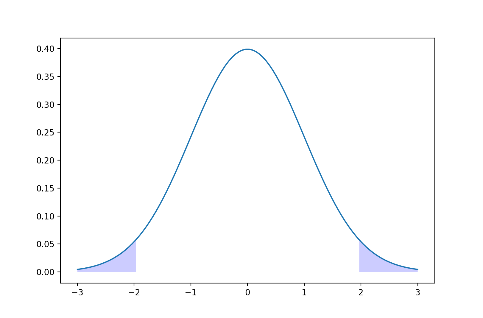
This “level of significance” is also known as $\alpha$, and is what affects how far away from the mean an observation has to be in order to constitute an anomaly. In a two-tailed test (an observation would be anomalous if it’s too far from the mean in BOTH directions) like this, the cut-off percentiles are simply $\frac{\alpha}{2}$ and $1 - \frac{\alpha}{2}$, which corresponds to the shaded blue regions above. What does it mean if we reject $H_0$ because we made an observation that lies in this region? It means that we’re correctly rejecting the null with probability $1 - \alpha$. There is always a probability of $\alpha$ that our null was true, and it was just due to sheer probability that our observation was that far from the mean, which, by definition, happens $\alpha$ of the time.

The $Z$ test can be done for any statistic, not just observations of data. As another example, suppose that we were trying to do linear regression of number of bathrooms ($X_1 \in \mathbb{R}^{n}$) and square footage ($X_2 \in \mathbb{R}^n$) to house prices ($y \in \mathbb{R}^n$) over a sample of size $n$. If we define our design matrix as one usually does in linear regression:

\[\newcommand{\mleft}{\left[ \begin{matrix}} \newcommand{\mright}{\end{matrix} \right]} \newcommand{\ones}{\mathbf{1}} \begin{align*} \mleft \vert & \vert & \vert \\ \ones & X_1 & X_2 \\ \vert & \vert & \vert \mright \end{align*}\]

Then our predicted covariate coefficients are simply: $\hat{\beta} = (X^\top X)^{-1} X^\top y$. A question one might ask is: how similar is our sample’s $\hat{\beta}$ to some presumed “null” $\beta$? I.E., if I had a strong reason to believe that houses in San Francisco related number of bathrooms and square footage to price via some $\beta$, do I have strong reason to believe that my sample came from the same distribution or otherwise? Then, notice that:

\[\hat{\beta} \sim \mathcal{N}(\beta, \sigma^2 (X^\top X)^{-1})\]

So the normalization of this would still be conceptually the same (subtract expectation, then divide by standard deviation):

\[\hat{\beta}_\text{normalized} = \frac{\hat{\beta} - \beta}{\sigma (X^\top X)^{1/2}} \sim \mathcal{N}(\mathbf{0}, \mathbf{I})\]

4. Deriving the $T$ statistic

The $T$ test, conceptually, has the exact same goal as the $Z$ test, the only difference is that we use the $T$ test only when we don’t know the population variance $\sigma^2$, which is a lot of the time. Very rarely do situations in real life allow us to know or even assume what the global variance $\sigma^2$ is. If we don’t have the variance, we have to at least estimate it somehow; if we don’t have ANY idea of how spread-out the distribution is, we can make no meaningful assessment of anomaly.

To estimate the population variance, we need multiple samples, not just a single data point. This is why a $T$ test is typically done on sample statistics (and not individual samples), such as sample mean $\overline{X_n}$, or even $\hat{\beta}$ as demonstrated in the example above. Before we deal with the fact we don’t know $\sigma^2$, let’s assume we know $\sigma^2$ and spell out clearly what it means to perform a test akin to $Z$ tests on a sample statistic.

Suppose we have a sample of $n$ data points $X_1, \cdots, X_n$, and we want to compare the sample mean $\overline{X_n}$ to a null (“presumed”) mean $\mu$. I.E., the null hypothesis assumes that:

\[\begin{equation*} X \sim \mathcal{N}(\mu, \sigma^2) \end{equation*}\]

This means that the sample mean has the following distribution:

\[\begin{align*} \overline{X_n} & \sim \mathcal{N}(\mu, \frac{\sigma^2}{n}) \\ \end{align*}\]

In the world of $Z$ tests, we wanted to normalize our distribution to a Standard Normal Gaussian because we have the $Z$ table for that, which makes it easy to get our percentile values (“$p$-value”). That is also true for the $t$ distribution; we have no analytical percentile function for it, but we do have numerical estimates of percentiles for a “standard” (actually, many, depending on degrees of freedom of the $t$ distribution, but more on that later) $t$ distribution. So, let’s normalize to try and get to as close to a Standard Gaussian as possible:

\[\begin{align*} \overline{X_n} - \mu & \sim \mathcal{N} \left(0, \frac{\sigma^2}{n} \right) \\ \Rightarrow \sqrt{n} \left(\overline{X_n} - \mu\right) & \sim \mathcal{N} \left( 0, \sigma^2\right) \\ \Rightarrow \frac{\sqrt{n}\left( \overline{X_n} - \mu\right)}{\sigma} & \sim \mathcal{N}\left(0, 1\right) \end{align*}\]

If we knew $\sigma^2$, that would be it. That’s exactly a Standard Gaussian, and we can just use the $Z$-test - we’re done. But, we don’t know $\sigma^2$, we only know $s$, which, in expectation, should be $\sigma$ (explicitly, $\mathbb{E}[s^2] = \sigma \Longleftrightarrow \mathbb{E}[s] = \sigma$), so perhaps we can just put $s$ in the denominator instead of $\sigma$ and call it a day. This would be our $T$ statistic that corresponds to this particular sample, but this is only halfway there, because unlike $\sigma$, $s$ is itself an observation of a random variable (sometimes, our sample has large variance (hence making $s$ large), sometimes, it has small variance (hence making $s$ small), but in expectation, the sample variance should be close to $\sigma^2$). To get our percentile, we need to know what the $t$ distribution is in order to see what percentile our $T$ statistic stands at. Now we have:

$T$ statistic

\[\begin{equation*} \frac{\sqrt{n}\left( \overline{X_n} - \mu\right)}{s} \end{equation*}\]

$t$ distribution

\[\begin{equation*} \Rightarrow \frac{\sqrt{n}\left( \overline{X_n} - \mu\right)}{S} \sim ? \end{equation*}\]

What is this? It’s a Standard Gaussian distribution over another random distribution. There are multiple ways to figure out what this is; you may write the whole thing out analytically and mash out the algebra, but the conventional way of doing it is to reason in terms of a $\chi^2$ (“Chi-Squared”) distribution. Notice that the numerator above has the following distribution:

\[\begin{equation*} \sqrt{n}\left( \overline{X_n} - \mu\right) \sim \sigma \mathcal{N}(0,1) \end{equation*}\]

The numerator is the Standard Gaussian scaled by $\sigma$. Our goal is to then express the denominator as something “standard”, also scaled by $\sigma$, so that the $\sigma$’s cancel out and our distribution becomes not a function of $\sigma$. Thankfully, there is some way to express $S$ just as that.

Finding the distribution of $S$:

We defined $S$ using a formula above, but let’s see what $S$ can also be written as:

\[\begin{align*} S^2 & = \frac{1}{n-1}\sum_{i=1}^n \left(X_i - \overline{X_n} \right)^2 \\ (n - 1)S^2 & = \sum_{i=1}^n \left(X_i - \overline{X_n} \right)^2 \end{align*}\]

Since $X_i$ are all i.i.d. and Gaussian, they can be written as a mean-centered multivariate Gaussian vector $W$:

\[\begin{align*} W = \mleft X_1 - \overline{X_n} \\ \vdots \\ X_n - \overline{X_n} \mright & = \mleft \mathbf{I} - \frac{1}{n}\ones \ones^\top \mright \mleft X_1 \\ \vdots \\ X_n \mright \sim \sigma \mathcal{N}(\mathbf{0}, \mathbf{I}) \end{align*}\]

We note down two important facts:

Firstly:

\[\begin{equation*}\sum_{i=1}^n \left(X_i - \overline{X_n} \right)^2 = \|X_i - \overline{X_n}\|_2^2 = \|W\|_2^2 \end{equation*}\]

is the sum of the squares of all the entries in $W$. If we rotate $W$ about the origin, the sum of squares will not change. $W$ is also a symmetric multivariate Gaussian ball, which is symmetric about the origin. So, we can simply rotate $W$ any way we want without changing the distribution nor the sum of squares.

Secondly:

\[\mleft \mathbf{I} - \frac{1}{n} \ones \ones^\top \mright\]

is a projection matrix that projects the $\ones$ subspace out of the operand.

If you combine the above 2 facts, we note that there is some way to rotate $W$ such that we can effectively just “nullify” one of the dimensions, making

\[\begin{align*} \|W\|_2^2 & = \sigma^2 (\text{the sum of }(n-1)\text{ squares of Standard Gaussian variables}) \\ & = \sigma^2 \chi^2_{n-1} \end{align*}\]

Wrapping this all together, we have:

\[\begin{equation*} S^2 = \frac{\sigma^2}{n-1} \chi^2_{n-1} \end{equation*}\]

$t$ distribution:

\[\begin{align*} \Rightarrow \frac{\sqrt{n}\left( \overline{X_n} - \mu\right)}{S} & \sim \frac{\sigma \mathcal{N}(0,1)}{\frac{\sigma}{\sqrt{n - 1}}{\sqrt{\chi^2_{n-1}}}} = \frac{\mathcal{N}(0,1)}{\sqrt{\frac{\chi_{n-1}^2}{n - 1}}} = t_{n-1} \end{align*}\]

The $t_{n-1}$ distribution, fully described as a “$t$ distribution with $n-1$ degrees of freedom”, is precisely defined as a Standard Gaussian over $\sqrt{\frac{\chi_{n-1}^2}{n-1}}$. You can see how expressing things in terms of scalar multiples of “standard” things like $\mathcal{N}(0,1)$ and $\chi^2$ allows us to cancel the $\sigma$’s in the numerator and denominator, effectively giving us a distribution that is not a function of $\sigma^2$. This is what makes the $t$-distribution and the $T$ statistic the hypothesis testing method of choice when we’re unable to make any assumptions on $\sigma^2$.

For visualization, here’s what the $t$ distribution looks like at various $n = $ degrees of freedom; image credits to Shoichi Midorikawa:

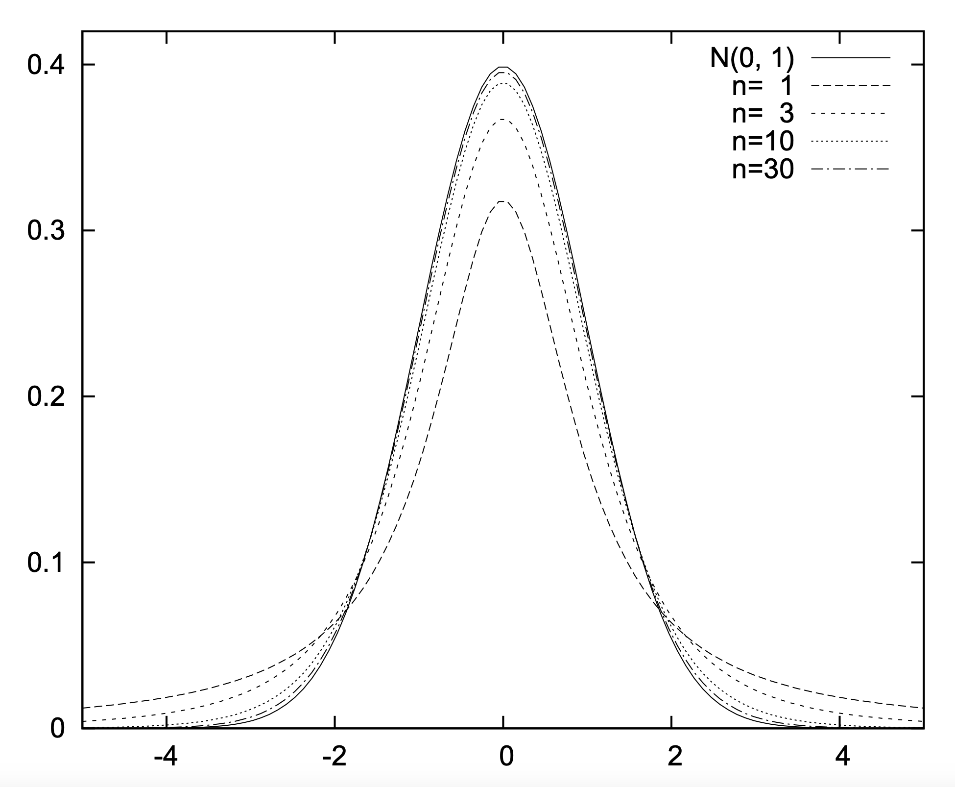
It looks very similar to the Gaussian distribution; as you can imagine, your $T$ statistic, will lie somewhere on one of these distributions (depending on degrees of freedom). While in the past, one might have used the $t$ table to figure out percentiles, now, you could easily do it using a programming language like R or Python.