Introduction

I recently came across an old lecture on High-Dimensional (HD) computing, in the forms of:

And thought it was a pretty interesting concept that tried to marry symbolic and empirical computation. To the uninitiated, “empiricism” largely refers to the current paradigm in AI - pure statistical fitting using universal approximation functions (neural networks), while symbolic computation refers to the old paradigm of AI, where people tried to build logic and structure into AI models, such as by programming grammatical rules into chatbots.

Symbolic computation has mostly died through the pre-2012 AI winter, but it’s making a return, and for various reasons, I’m also a huge proponent of it. Even people in the empiricism camp cannot deny that the type of work involved in symbolic computation - designing computational structures that will be more amenable to certain types of learning (e.g. learning inductive relationships, learning spatial patterns, etc.) and knowledge encapsulation - is unavoidable even in the current paradigm of AI. As a simple example, one can consider that the differences between MLPs, CNNs, and RNNs, are chiefly that the differences in their architecture allow different types of patterns (local spatial patterns, inductive recurrent patterns, etc.) to be more easily learnt.

This post aims to be a simple summary of the lecture above, and to quickly explore some comparisons between this flavor of symbolic computation (HD computing), and the current state of AI, which also uses lots of high-dimensional vectors. It will mostly be a summary of Pentti’s lecture.

Preamble: Today’s AI

Vector Spaces and Concepts

As preamble, it’s worth going through the overarching characteristics of the information that models today can learn, and how they are expressed.

Models today often take an input vector, encode / embed it into some lower-dimensional vector space (these hidden vectors are called “embeddings”), pass them through several blocks (usually transformer / CNN / MLP) to transform said embeddings, and then finally, decode them into the same domain as the input (e.g. one-hot vectors representing words / tokens, or images, classification vectors, or whatever else). Because these embeddings are lower-dimensional than the inputs, and are intermediate representations of the data, it is inevitable that they contain a more efficient representation of the data. In other words, these embeddings represent higher-level abstract concepts that the model has learnt are the most discriminating features that allow it to best perform the task it was trained to perform.

If this all sounds abstract, then here is an example. In a contrived example where we generated random static noise fields in green and red, and trained a small MLP to classify green static noise images as class A and red as class B, it makes sense for any model to simply learn that if the G channel is highly active, then it’s class A, else it’s class B. In a very small MLP, where the size of the hidden dimension is 2, it is inevitable that one of the elements of this vector will have a very high value (a.k.a “the neuron will be highly activated”) when the G channel is highly active, and the other will be highly activated when the R channel is highly active. We say, in this case, the model has learnt to represent greenness and redness, and there is a linear mapping that corresponds to greenness and redness in one of its embedding spaces.

In a larger MLP, this representation is not inevitable, because the model could just learn to capture some spurrious correlation between noise and the various classes, just by sheer probability. In the extreme case of a huge model, the model could essentially just memorize the training examples. Thankfully, there is little incentive to create such over-parameterized models as they are computationally expensive, and modern-day problems (e.g. language) are so huge and complex that the sizes of the latent spaces of today’s SoTA models are comparatively small, and encourage the learning of concepts, rather than memorization.

Latent Spaces are linearly mapped to Concepts

Through a handful of really interesting, intuitive, and replicable papers, we have learnt that today’s models do indeed learn concepts, and represent them linearly in their latent spaces. From the famous King - Man + Woman = Queen finding, to this paper on thought vectors, to this marvelous study of interfering though vectors, and so many more papers, we have found that semantic meanings can largely be mapped to certain directions in latent space. And these are not just toy experiments either - Anthropic (creator of Claude) dove into their models and gave us a dictionary of neuron-to-meaning mappings, and DeepMind also came up with a way to force a model to learn linear mappings of meanings that they found was similar to the way monkeys represented visual information.

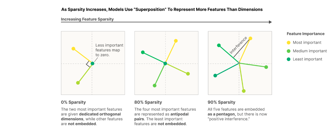Latent semantic vectors when you try representing 5 concepts in 2 dimensions (Anthropic)

So that’s really the punchline I wanted to arrive at in this preamble - present-day AI models already learn to represent meaning as directions in vector-space. Now, we can jump into HD computing.

Pentti’s Lecture Summary

Pentti’s lecture aims to introduce HD computing as a way to represent arbitrary information in high-dimensional vector space TLDR. This approach allows one to

Simultaneously store various information pieces in the same aggregate vector (superposition)
Given an aggregate vector and query vector, recover constituent pieces of information
Learn concepts (I think of this as a linear mapping of meaning to some high-dimensional subspace) data-efficiently, and compute-efficiently.

Embedding Meanings: Pentti’s Trigram Example

To start, Pentti walks through a Trigram example, which introduces an algorithm which:

Can embed a sentence into a vector.
This sentence vector can serve as a vector for a language (called “Language Profile”).
In a test of randomly chosen Language Profiles of 21 EU languages, when comparing a test set of 21,000 test sentence vectors (1,000 per language) to these Language Profiles, the closest match was the correct language 97.3% of the time.
This vector embedding scheme can also predict the next alphabet / token.

In the lecture video, Pentti first introduces the idea of encoding sequences by doing rotation operations (more accurately, permutations) on the constituents of the sequence, and then point-wise multiply them. For example, to encode the sentence THE, we simply rotate the vectors of each letter by a number of times depending on its position in the sequence - in this case, T is rotated twice, H is rotated once, and E not at all, and point-wise multiply all of them together. The vectors for each individual letter are just randomly sampled 10,000-vectors $\in \{1, -1\}^{10000}$. Here’s a screenshot from the video:

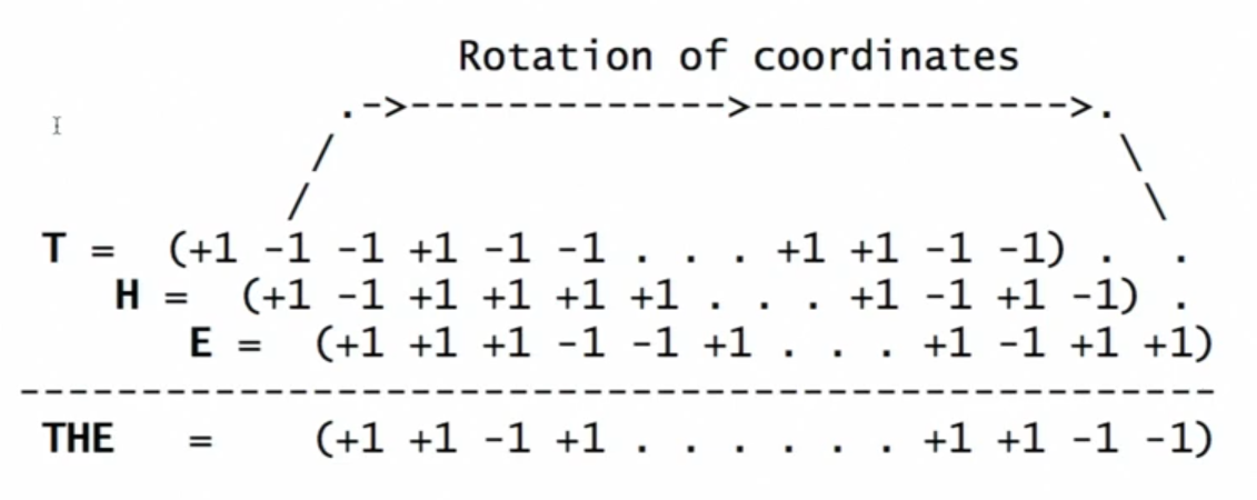
So in essence, this operation can be denoted as follows:

\[\begin{align*} \phi(THE) = \left[ R^2 \cdot \phi(T)\right] \odot \left[ R \cdot \phi(H) \right] \odot \phi(E) \end{align*}\]

where $\phi$ denotes the vectorize representation of its operand, and $R$ is a permutation matrix that looks like:

\[R \in \mathbb{R}^{10000 \times 10000} = \begin{bmatrix} 0 & 0 & \cdots & 0 & 1 \\ 1 & 0 & \cdots & 0 & 0 \\ 0 & 1 & \cdots & 0 & 0 \\ 0 & 0 & \cdots & 0 & 0 \\ & &\cdots \\ 0 & 0 & \cdots & 1 & 0 \end{bmatrix}\]

Language Profile (LP)

Having a way to:

Generate letter embeddings ($\phi$, which is random)
Generate trigram embeddings

We can simply construct an LP by rolling a trigram computation window over any randomly selected sentence, and summing up all the trigram embeddings. For example:

\[\begin{align*} \phi(\text{THE QUICK..}) = \phi(\text{THE}) + \phi(\text{HE }) + \phi(\text{E Q}) + ... \end{align*}\]

And what you get is basically a vector (the LP) representing a histogram of trigrams. To make it easier to get an intuitive understanding of this fact, I point out that:

Since $\phi$ is a randomly sampled vector $\in \{1,-1\}^{10000}$, then $\phi$ has some random direction, but its magnitude is always $\sqrt{10000}$.
As the dimensionality of the subspace increases, the probability that any 2 randomly sampled vectors is almost orthogonal approaches 1. Therefore, it is almost certain that all trigrams have orthogonal directions. The LP vector hence can be decomposed into a linear combination of the orthogonal trigram vectors that make it up, where the coefficients are the approximate (but very nearly exact) counts of each trigram.

Next Token Prediction: Randomness Saves The Day

This example mainly just serves to illustrate that in high dimensions, so long as you have SOME relationship built into your vectors, finding two related meanings / vectors (needle-in-a-haystack) is feasible, by the grace of the probability gods.

This LP / trigram embedding scheme also allows you to query the most likely next-letter, given a bigram. For example, you may ask the question: in English, what’s the letter most likely to follow $\text{TH}$? This is how Pentti proposes to find it:

\[\begin{align*} \text{Let } Q & = \left[ R^2 \cdot \phi(\text{T}) \right] \odot \left[R \cdot \phi(\text{H})\right]\\ \text{Let } \text{LP} & = \text{LP for English} \\ X & = \text{letter whose } \phi \text{ has smallest cosine dist to } Q \cdot \text{LP} \end{align*}\]

How does this make sense? I actually don’t think this makes sense, but perhaps it works with high probability due to how these vectors are distributed in high-dimensional space. Here’s why it does not make sense to me:

First, we do $Q = \left[ R^2 \cdot \phi(\text{T}) \right] \odot \left[ R \cdot \phi(\text{H})\right]$. Then, based on how we computed the trigrams, we can say that if $\text{THX}$ is part of English, then $Q \odot \phi(X)$ should look somewhat similar to $\text{LP}$. That is:

\[Q \odot \phi(X) \approx \text{LP}\]

More specifically, $Q \odot \phi(X)$ likely LESS orthogonal to $\text{LP}$ than any other randomly selected vector, since any randomly selected vector is almost completely orthogonal to any other vector in high-dimensional space. Why is this true? Remember how we constructed the language profile:

\[\begin{align*} \text{LP} & = n_A \cdot\phi(\text{trigram A}) + n_B \cdot \phi(\text{trigram B}) + \cdots + n \left(Q \odot \phi(X)\right) + \cdots \end{align*}\]

where the various $n$’s are just integer multiplicities reflecting how many times each trigram occurred in the language profile sentence. In particular, there is a non-trivial component of $\text{LP}$ in the $Q \odot \phi(X)$ direction.

From here, it makes sense to construct the following:

\[\begin{align*} Q \odot \phi(X) & \approx \text{LP} \\ \Rightarrow \phi(X) & \approx Q^\Theta \odot \text{LP} \end{align*}\]

where $\Theta$ denotes the Hadamard Inverse. How Pentti dropped the inverse there, I do not know. However, there is an interesting property between:

$Q \odot \text{LP}$
$Q^\Theta \odot \text{LP}$

Since $Q^\Theta$ is an element-wise inverse of $Q$, it means that every element of both vectors have the same sign. This means that $\angle (Q \odot \text{LP}, Q^\Theta \odot \text{LP}) \leq 90^\circ$. This is significantly NOT orthogonal (relative to random vector pairs) in high-dimensional vector spaces.

There is a further rather amusing effect. If two vectors $a$ and $b$ are not orthogonal, and $b$ and another vector $c$ are not orthogonal, then it is likely that $a$ is not orthogonal to $c$. Probabilitistically speaking (and I have yet to prove this rigorously, but just from my imagination and running simulations, it seems true), the higher the dimensionality, conditioned on $\angle (a, b) \leq (90 - \varepsilon) ^\circ$ and $\angle(b, c) \leq (90 - \varepsilon) ^\circ$, the more likely $\angle (a, c) \leq (90 - \varepsilon) ^\circ$.

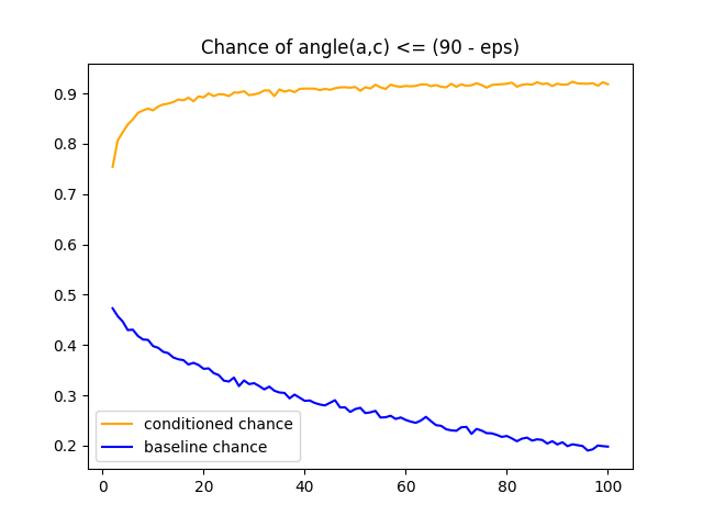Chance of non-orthogonality over dimensionality

Let $a = Q \odot \text{LP}$, and $b = Q^\Theta \odot \text{LP}$, then we have $\angle(a,b) \leq (90 - \varepsilon)^\circ$. Let $c = \phi(X)$, then we have $\angle (b, c) \leq (90 - \varepsilon)^\circ$. Then, we have the above effect, which is the most amusing. This explains why Pentti’s next-token prediction math works out even though the Hadamard inverse is missing - it is just statistically true most of the time, and “most of the time” becomes overbearingly “most of the time” the higher the dimensionality of the vector space.

So as you can see, the Hadamard product and high dimensionality gives us some very nice properties that allow us to retrieve related information. Going back to the big picture, the overarching takeaway here is that in high-dimensional subspaces, any independently sampled vector is always almost orthogonal. If you wanted to do information retrieval from a “database” (in this case, $LP$) using a query vector (in this case, $Q$), so long as $Q$ and $LP$ are “similar” (i.e. are not almost orthogonal, i.e. a significant component of both vectors lie in the same direction), you can almost certainly do it.

Superposition of Information

In fact, we saw that because any 2 random vectors in a high-dimensional subspace are likely “dissimilar” (nearly orthogonal), if we have multiple pieces of information we wish to store, we could store them in the same vector. This is because the vector that encodes any two unrelated pieces of information are likely also dissimilar. This means that the two pieces of information will lie predominantly in mutually orthogonal subspaces.

He introduces how this may be done by exmplifying how one may store a dictionary (key-value pairs). This time, he switches the vectors to be randomly sampled $\in [0,1]^{10000}$ in order to emulate bit arrays. The only interesting parts here are:

The introduction of a binding operation (XOR, which is its own inverse), that allows us to bind a key vector to a value vector, as in $\phi(K \rightarrow V) = \phi(K) \oplus \phi(V)$.
The combination of all key-value pairs into a single bit-vector by using the $\text{Majority}$ operator, as in $\phi(\text{Dictionary}) = \mathbf{1} \left\{ \left[ \sum_{i}^N \phi(K_i \rightarrow V_i) \right] > \mathbf{\frac{N}{2}} \right\}$. In English, the $\text{Majority}$ operator simply switches on the bit in that position if the value of that bit is greater than $N/2$ post-summation.

The rest of the example essentially just demonstrates how the magic of everything-is-almost-orthogonal-in-high-dimensionality is able to nullify the problem of interference introduced by the $\text{Majority}$ operator and allow us to do correct information retrieval almost all the time. I won’t dispute what is meant by “almost all the time,” as researchers have shown that this quite a robust measure.

The major caveat is that to do information retrieval, you have to store all the vectors that you could possibly want to retrieve, as the retrieval algorithm is essentially a nearest-neighbor problem.

Comparison with Transformers and present-day AI

So here Pentti outlines the key similarities between HD computing and Deep Learning (DL):

Both learn statistically from data
Both can tolerate noisy data
Both use relatively high-dimensional vectors (DL algorithms slow down significantly though)

And the key differences:

HD computing is founded on “rich and powerful mathematical theory” rather than on heuristics
New codewords (read: semantic vectors) are made from single application of HD vector operations ($\odot, \oplus, \text{Majority}$)
HD memory is a separate function (you have another agent that is in charge of storing data and retrieving best matches to queries using nearest-neighbor search)

And the result is that HD computing is transparent, incremental (on-line), and scalable.

Before we interrogate this comparison, let’s keep in mind that this lecture was in 2017, the very same year that Transformers first got invented, and certainly way before interpretability research uncovered neat properties of embeddings learnt by DL models.

“Rich and powerful mathematical theory”

I think this conclusion stems from the fact that we know that in high-dimensionality, every randomly sampled pair of vectors is almost guaranteed to be dissimilar. We then can decide that semantic vectors will be set to randomly sampled (dissimilar) vectors. The result is that we then know that if two unseen vectors are dissimilar, then they must represent different concepts. To that, here are my retorts:

The hadamard product ($\odot$) gives us a nice way of almost always generating a new dissimilar vector from 2 input vectors. However, there is no geometric meaning to the hadamard product, and it is also not guaranteed that this operation will always uphold the “new codewords are made from single application of HD vector operations” property. For example, what if one of our vectors was the $\mathbf{1}$ vector or the $\mathbf{-1}$ vector? In general, there is also no proof that for any special class of vectors (binary, since such vectors will be stored using bits), $\forall \{a, b, x, y\} \text{ s.t. } \{a,b,x,y\} \text{ are dissimilar }, \Rightarrow a \odot b \text{ and } x \odot y \text{ are dissimilar}$. Until this property (seems to be an isomorphism we want) is proven or even shown to be the statistical inevitability as dimensionality increases, I’m not sure this is a watertight argument.
We know now that lots of superpositions happen in the embedding space of DL models. Concepts are mapped to directions in the embedding space, much like how they are assigned to orthogonal vectors in HD computing. If there are sufficient dimensions in the embedding space, each concept will get a privileged basis vector (the standard basis vectors, which are orthogonal!). If there are insufficient dimensions, then the concept vectors are organized into an arrangement that spaces them out as much as possible (maximizes orthogonality). Read Anthropic’s Toy models of superpositions paper for more details.

So, the main difference seems now not to be that we know properties about HD computing vector spaces and not about DL vector spaces, but that the HD computing vector spaces are pre-determined, whereas DL vector spaces are learnt. Well then, it’s not clear what benefits HD computing can bring us in this case, because to use HD computing, we have to know what concepts there are that we need to represent ahead of time. This is very much the problem of feature engineering being futile; we should let black-box models learn what these features are and tell us!

“New Codewords are made from application of HD vector Operations”

I really like this property. The fact that you can operate on a vector and arrive at a different vector in the same subspace with a different meaning is really cool. The fact that the entire model also only uses this one vector subspace is really cool. Despite the above retort on these operations not necessarily being isomorphisms, I think the idea of having one large subspace represent the entire latent space (rather than DL models having multiple latent spaces due to having multiple layers) is really cool, and feels closer to how our brains encode information. This is because having one latent space represent everything forces the model to consider all concepts / features as equals, no matter how high-level or low-level each may be. For example, in CNNs, edges are low-level features, while shapes are higher-level features. These features do not appear in the same layer, and are hence not in the same latent space. When such information is synthesized, they are symmetric.

However, I think that things like skip-connections and Transformer residual streams support the notion that having one unified latent space is very beneficial. There is a possible research question worth exploring: what if we structured neural networks to have one big recurrent block as opposed to multiple successive blocks?

“HD memory is a separate function”

Now I’m not sure what the perk of this is. Having to store all your data (train AND test) seems to be a con, no matter how you twist it. Don’t have much to say here.

Conclusion

HD computing presents merely a different way of doing things. It doesn’t seem to bring any compelling property to the table in order to achieve greater transparency or efficiency, or expressiveness that DL models already give us.

High Dimension Computing