Many time-series tasks share the ability to decompose (e.g. using the Fourier Transform) and express data using spectrograms. Could this, in and of itself, be a sufficient form of “shared structure” that could allow us to train a multitasking model that can essentially transfer-learn knowledge across different time-series problem domains for better classification performance?

A Stanford Multitask, Meta-Learning (CS 330) research project done in collaboration with two colleagues. Contact me for more information!

Abstract
Introduction
Related Work
Datasets and Preprocessing
Methods
Experiments
Results / Discussion
Conclusion / Future Work
Litmus Test: EEG Classification
References

1. Abstract

1.1 Motivation

There is an abundance of important classification tasks across various time-series domains, such as speech classification, noisy audio recognition, EEG recording analysis, digital signal processing in dense environments, etcetera. Many of the techniques used involve an intermediate step of discretizing the time-series into discrete frequency buckets and time-steps. Indeed, we realize that all of these tasks may have the potential to share a similar structure if expressed as spectrograms and, more specifically, Mel-Frequency Cepstral Coefficients (MFCCs), which are visual representations of a signal’s frequency spectrum as it varies with time.

This is reason to believe that applying fine-tuning and transfer learning amongst these different time-series problem domains might uncover this potential shared structure and lead to better classifiaction performance on downstream tasks. In this paper, we investigate a method for using transfer learning amongst speech, audio, EEG, and digital signal data using spectrograms and MFCCs. We show that by training a deep convolutional neural network on one type of data and then fine-tuning it on the other types, we can achieve improved performance and quicker convergence compared to training a network from scratch.

1.2. Summary of Methodology

Summarily, our experimental steps can be enumerate as follows:

We produce a baseline result by shortlisting a small set of classification tasks and their corresponding training data, and then training a fixed, chosen model (albeit with different final classification layer) on each of these tasks alone.
We then explored transfer-learning from one task to another on all permutation pairs of tasks in the same set of tasks and compared them to the baseline.

1.3. Summary of Findings

We found that transfer learning can be helpful (outperform baseline), and is at worst, not destructive; this is in the sense that if the task at hand has inadequate data, transfer learning is beneficial, but if the task at hand has adequate data, transferring from another task can delay convergence, but does not prevent or significantly delay it.

In this sense, we have found that spectrogram tasks across domains do indeed have some shared structure, but their differences are significant enough that prevent us from being able to generalize them simply as “spectrogram tasks”. In transfer learning from one spectrogram task to another, there is often a trade-off between choosing a source task with a large dataset and a more “similar” source task, which, by virtue of being similar, does not usually have a substantially larger dataset than our actual task of interest.

2. Introduction

To reiterate, our project is motivated by the fact that a lot of time-series tasks share the ability to decompose (via things like Fourier Transform) and express data using spectrograms and MFCCs. We proposed that there may be a potential shared structure between these spectrograms that can benefit from the ideas and techniques of transfer learning and lead to better classification performance across these tasks, which is what this paper explores.

Transfer learning is a powerful technique that has been widely used in many areas of machine learning, including computer vision, natural language processing, and speech recognition. It involves training a model on one task and then fine-tuning it on a related task, using the knowledge learned from the first task to improve the performance on the second task.

To summarize, in this paper we apply transfer learning to the problem of analyzing speech, audio, EEG, and digital signal data. We represent all of the data as spectrograms (more specifically, MFCCs, which you may think of as a more human-natural version of a simple Fourier Transformation as one of the added steps involves taking the log of the amplitudes for each frequency), visualizations of a signal’s frequency amplitudes over time. Since these spectrograms are essentially images, it is easy for us to use a Convolutional Neural Network (CNN) to learn all tasks, hence allowing us to easily transfer-learn across tasks, if possible.

Review of papers allowed us to conclude that the use of MFCCs and CNNs was viable.

In the paper “Abnormal Signal Recognition with Time-Frequency Spectrogram: A Deep Learning Approach” by Kuang et al. [2022], researchers were able to successfully show that transforming time-series input signals to spectrograms and using an image classification model was a viable and good approach to recognize abnormal signal patterns, even in a dense signal environment and with low Signal-to-Noise-Ratio (SNR) conditions.
A similar approach was also shown in the paper “Signal Detection and Classification in Shared Spectrum: A Deep Learning Approach” by Zhang et al. [2021], where the team decided to batch segments of received Wi-Fi, LTE LAA, and 5G NR-U signals in the 5-6 GHz unlicensed band, pass spectrograms of the input to a model that is combined with a Convolutional Neural Network layer and a Recurrent Neural Network layer to perform signal recognition, and were able to show good detection and high accuracy with many coexisting and similar digital signals.
In addition, the paper “SSAST: Self-Supervised Audio Spectrogram Transformer” Gong et al. [2021] improves upon the Audio Speech Transformer model, which is a transformer model that performs audio classification with spectrograms as the main input source, specifically by leveraging self-supervised learning using unlabeled data from both speech and audio. It proposed to pretrain the AST model with joint discriminative and generative masked spectrogram patch modeling (MSPM) using unlabeled audio from AudioSet and Librispeech, and was able to get state of the art benchmark results.

All of these papers suggest that spectrograms and MFCCs would provide a good approach towards the our time-series classification task, and the last paper suggests that using multiple data sources may help transfer a shared structure and improve performance.

4. Datasets and Preprocessing

We decided to work with the following datasets for our project:

UrbanSounds8K (Audio) Salamon et al. [2014]:
- A 10-way classification dataset consisting of 8,732 urban sounds, such as “dog bark” or “siren”.
PanoradioHF (Digital Radio) Scholl [2019]
- An 18-way classification dataset of 172,800 digital signals labeled according to its transmission mode, such as “morse”, “fax”, or “psk31”. Each signal had a sampling rate of 6000 Hz and had varying center frequency offsets and SNR values ranging from 25 to -10 dB.
AudioMNIST (Speech) Becker et al. [2018]:
- A 10-way classification dataset consisting of around 30,000 sample recordings of people saying the numbers 0 to 9.
Grasp-And-Lift (EEG) Kaggle [2015]:
- A 6-way classification dataset of 3,962 32-channel EEG signals corresponding to when a person is trying to lift their hand, release grip, etc.. We mean-ed all the 32 channels into a single channel time-series data.

For brevity, we simply refer to the above datasets by the names written in parentheses, e.g. “Audio” refers to UrbanSounds8K and “Speech” refers to AudioMNIST.

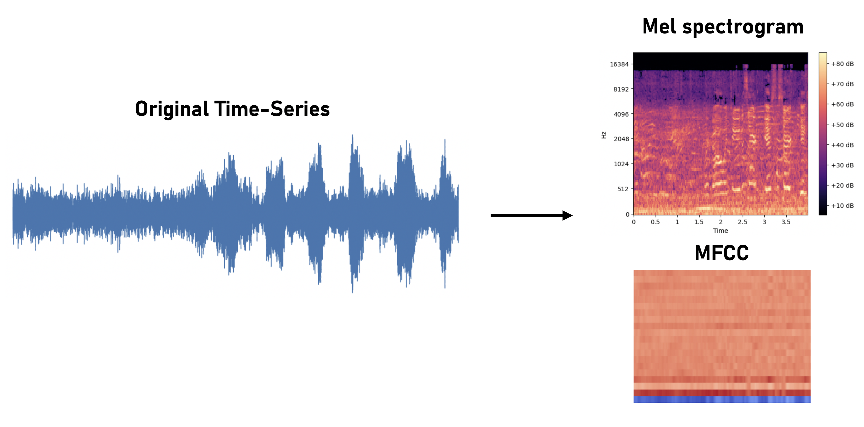
For all of our datasets, we converted the time-series waveforms into mel spectrograms and MFCCs.

Mel spectrograms and MFCCs are commonly used in audio classification tasks as they provide a good visual representation of the spectrum of frequencies of a signal as it varies over time.

To convert time-series data into spectrograms, we:

Divide the signals into segments of a fixed length window and apply a Fourier transform to each segment in time, resulting in a matrix where each column represents the frequency spectrum of one segment of the original signal.
Generate MFCCs by performing a Discrete Cosine Transform on the mel spectrogram, extracting useful features for audio and speech while also reducing data dimensionality.

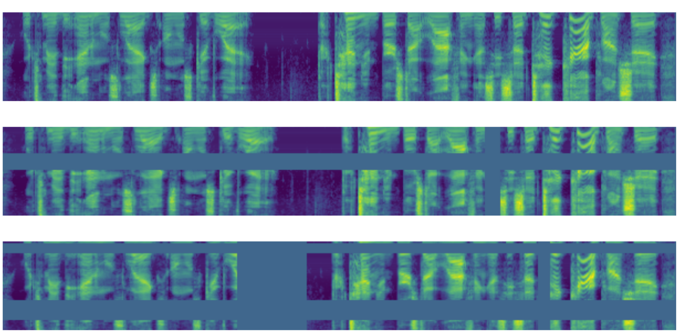
Throughout our research and experimentation, we learned that using an image-based approach towards audio classification and these other types of time-series tasks tends to be prone to overfitting. Because of this, we decided to implement SpecAugment, a data augmentation method for speech recognition that warps spectrogram features as well as masks blocks of frequency and time steps. The development of this method by Park et al. [2019] was proven to help reduce overfitting and resulted in more generalizable models, and an example of the spectrogram that this technique generates is shown in the figure below.

5. Methods

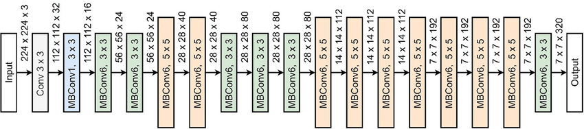
For this project, our team decided to use the EfficientNetB0 model architecture by Tan and Le [2019] as the base model for the various time-series classification tasks. This model has been shown to achieve good performance on a variety of image classification benchmarks, and thus we believed it would be a suitable starting point for our approach of using spectrograms and mfccs. A diagram of the layout of the EfficientNet model is shown in the figure below.

For each of our classification tasks that we chose, each sample only belonged to a single class label, so using categorical cross-entropy as our loss function was natural:

\[Loss = - \sum_{i=1}^{n_{classes}} y_i \cdot \log{ \hat{y}_i}\]

6. Experiments

6.1. Baseline, then Transfer

Once we preprocessed all of our datasets and converted everything to spectrograms and MFCCs, we were then able to start training our networks and testing out various techniques relating to the ideas of transfer learning and fine-tuning. We started our experiments by training the network on just one type of data, such as the urbansound8k speech data, which served as our baseline (i.e. no pretraining). Then, we used those trained model weights to conduct fine-tuning on the other tasks in a pairwise fashion, including audio, EEG, and digital signals. This approach allowed us to observe if the network could learn general features from the initial training data and then transfer these features onto the fine-tuning data to improve performance or lead to quicker convergence.

6.2. Multitask Learning Tricks

Freezing Layers

We also experimented with the amount of layers we chose to freeze, or not update, during fine-tuning, with the goal of trying to see at which layers the model was able to extract the most useful features from the initial training data, and see if there was any intuition behind it. There are a total of 80 conv2d layers in EfficientNetB0, not including the first input layer and last classification layer, and we wanted to investigate how freezing different numbers of these layers would affect the model’s performance. To this end, we conducted experiments where we froze the first 60 conv2d layers, then the first 30 conv2d layers, and finally the first 10 conv2d layers. This allowed us to see how the model performed when given more or less freedom to adjust the weights of the conv2d layers during fine-tuning.

Mixing Tasks

Lastly, we decided to train a model with a combination of our datasets mixed together. Specifically, we combined the Audio dataset, Speech dataset, and Radio dataset into one large dataset with a new combined total of 38 classes. We created MFCCs of the same exact size, 20 mfccs $\times$ 61 time-steps $\times$ 1 channel, for each of the training examples, and also performed specAugment on all of the data in order to get a more even distribution of classes. The goal of this model was to see if training multiple time-series tasks in one model would lead to better performance on held-out test sets for each individual task compared to the from-scratch models and the other pretrained models, and to serve as another way to observer any potential shared structure between the data domains.

7. Results / Discussion

By comparing the performance of the frozen and unfrozen layers, we were able to identify the layers that were most important for learning the common structure shared by the datasets. We used a variety of techniques to compare the performance of the frozen and unfrozen layers, including visualizing the learning curves, calculating the average training and validation loss and accuracy, and performing statistical tests to assess the significance of the differences. We also employed a range of hyperparameter tuningtechniques for training the networks, such as adjusting the learning rate and regularization parameters and using data augmentation and dropout to prevent overfitting. After training each network, we evaluated its performance on sets of held-out test data to see how well it performed on unseen examples, using accuracy as our main metric for comparing the results.

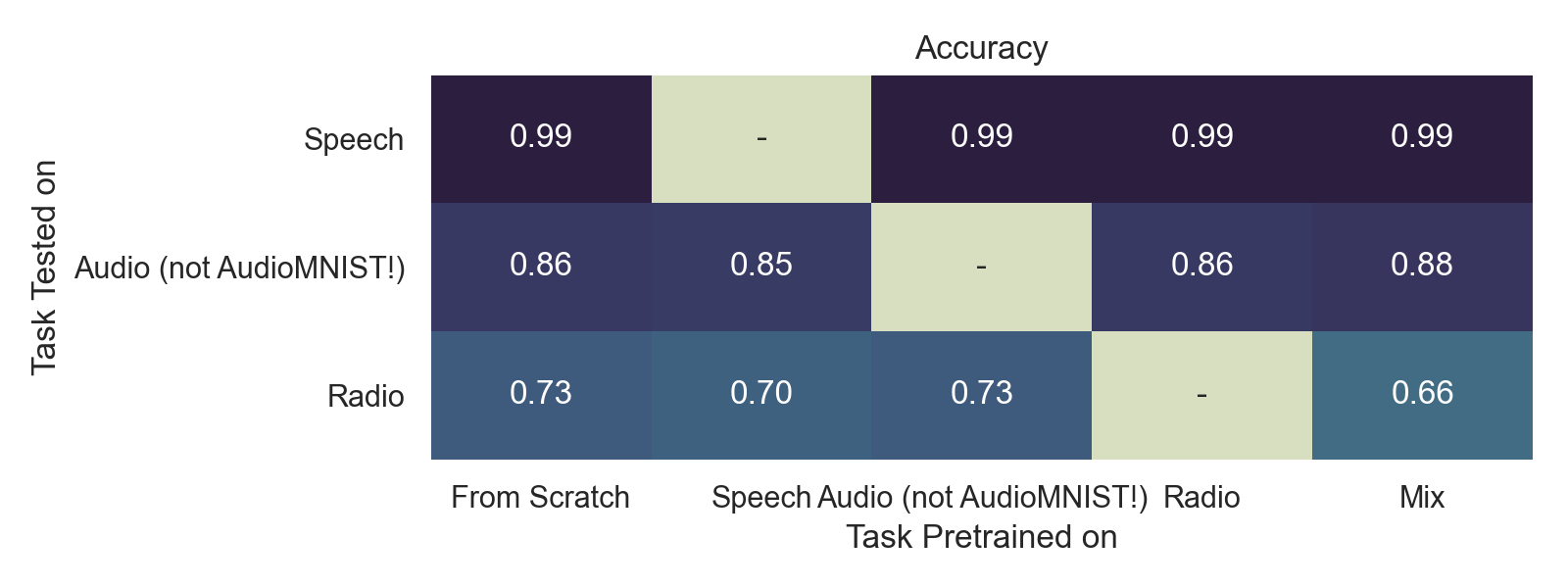
7.1. Accuracy on various datasets / pretraining

Here, we treat the accuracy of the model that is trained from scratch as the baseline. It may not be very insightful for certain configurations as this table reports peak performance, which, for some datasets, is the same for all configurations as the model is generally able to eventually get to the same level of good performance (essentially 100% accuracy). We hence also show our loss curves to compare convergence rates.

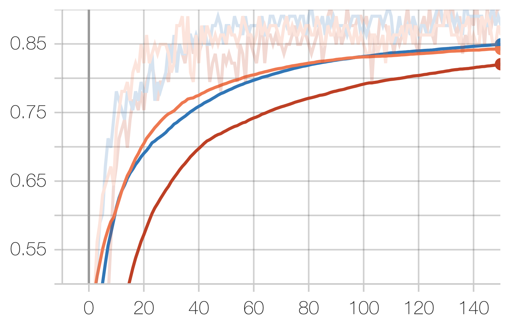
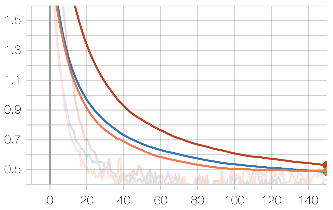
7.2. Convergence Curves

Audio Task:

Legend: Scratch, Speech, Radio

Audio Accuracy Curves (test split)

Audio Loss Curves (eval split)

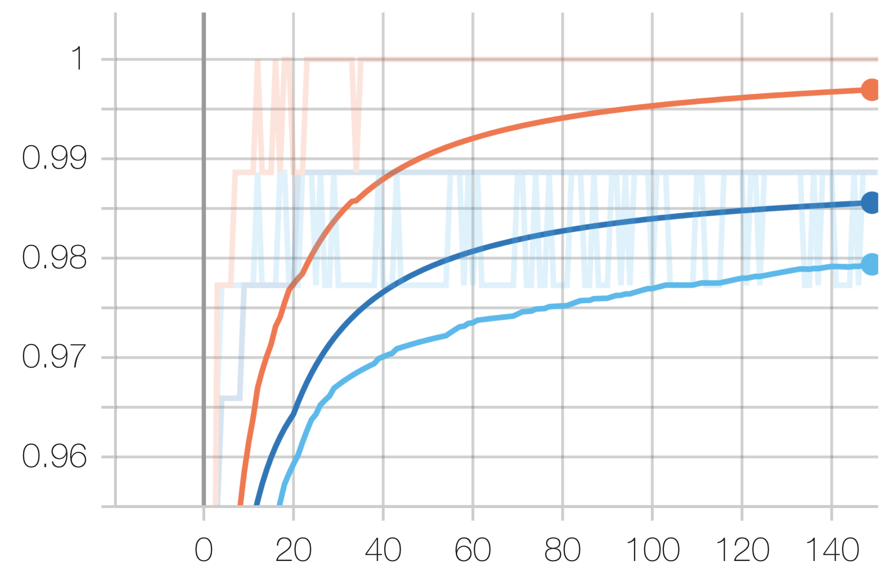
Speech Task:

Legend: Scratch, Radio, Urban

Speech Accuracy Curves (test split)

Speech Loss Curves (eval split)

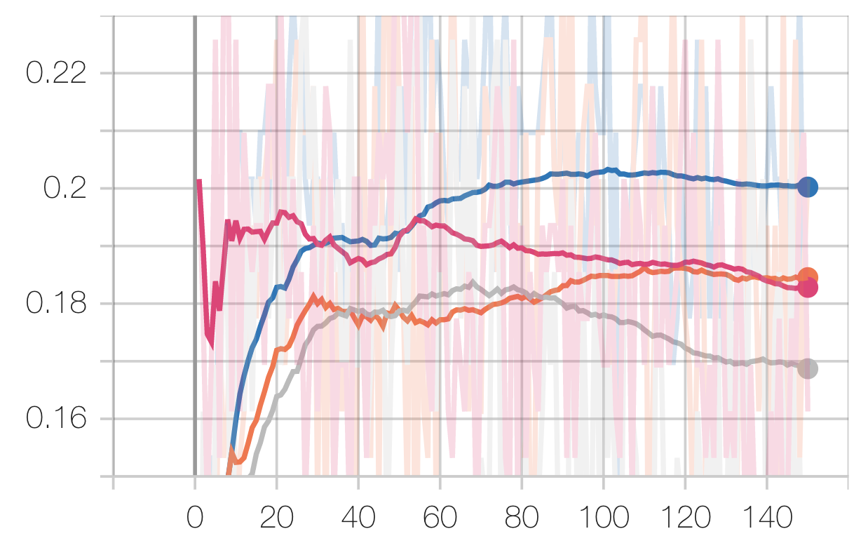
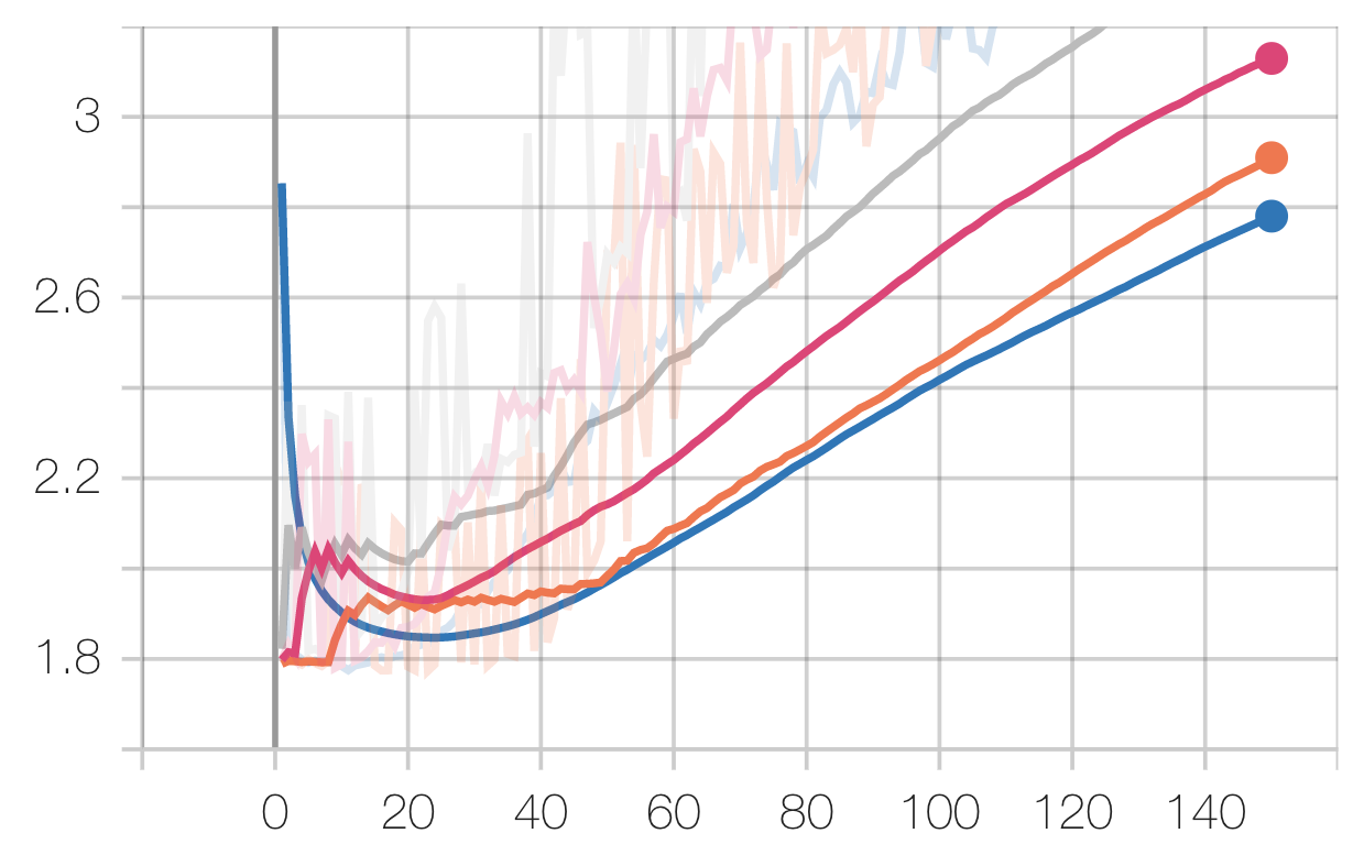
Radio Task:

Legend: Scratch, Speech, Audio

Radio Accuracy Curves (test split)

Radio Loss Curves (eval split)

Note that while our experiments do not care about our technique’s performance in relation to the start-of-the-art, it is insightful in allowing us to draw conclusions about the nature of spectrogram tasks.

8. Conclusion / Future Work

To summarize, there is some shared structure between time-series spectrogram tasks, but our findings can be broken down into three categories of insight, as explained below.

8.1. Dataset Size

If the task has adequate data, training-from-scratch usually yields the best results. Observe that the reported accuracies for each of the tasks above were highest for the training-from-scratch configuration, except for the audio task (smallest dataset) and the EEG task. The fact that the audio task performed better with pretraining suggests that its dataset was small and benefited from pretraining on a larger dataset. However, this is most definitely a trade-off between the gain from pre-training on a large dataset, and the cons of doing most of the training on another dataset with potentially large task / distributional differences. We shall see this in the later section on EEG classification.

8.2. Direction of Transfer

It was also found that transferring is not bijective (i.e. pretraining on $\mathcal{T}_A$ and transferring to $\mathcal{T}_B$ is different from pretraining on $\mathcal{T}_B$ and transferring to $\mathcal{T}_A$).

Another interesting thing to note is that pretraining did not necessarily lead to faster convergence. In fact, it seems that pretraining may sometimes delay convergence, indicating that different spectrogram time-series tasks have meaningful structural differences; they cannot be generalized simply as “spectrogram time-series tasks”.

8.3. Multitasking Ability

We don’t believe our experiments reach any conclusive results on the multitasking ability of one model on multiple different datasets. We can see that mixing multiple tasks into 1 super-task, pretraining on that super-task, and transferring to another metatest task, does not necessarily yield better or worse results (outperformed all other pre-training configurations and transfers to audio, but outperformed by all other pre-training configurations and transfers to radio). We think that this is an interesting area for future exploration, but definitely that more work has to be done to establish the relationship between task mixing and performance, while controlling for other factors like dataset size.

In conclusion, we were able to find that there is some common structure between the time-series datasets and like to fine-tune deeper by freezing different layers in the model to save those common structures and save more resources when training.

Perhaps as a litmus test for ourselves, we wanted to do some preliminary investigation of transfer-learning onto an EEG task, which is a particularly valuable application of our work as EEG data is very scarce. We wanted to complete the same experiments on the EEG dataset, which, based on our preliminary trials, we have reason to believe will yield good results.

9. Litmus Test: EEG Classification

Since transfer learning across spectrogram tasks did prove to work in some scenarios, we have reason to believe that transferring to EEG dataset would work. We hence explored the performance of various transfer sources versus baseline:

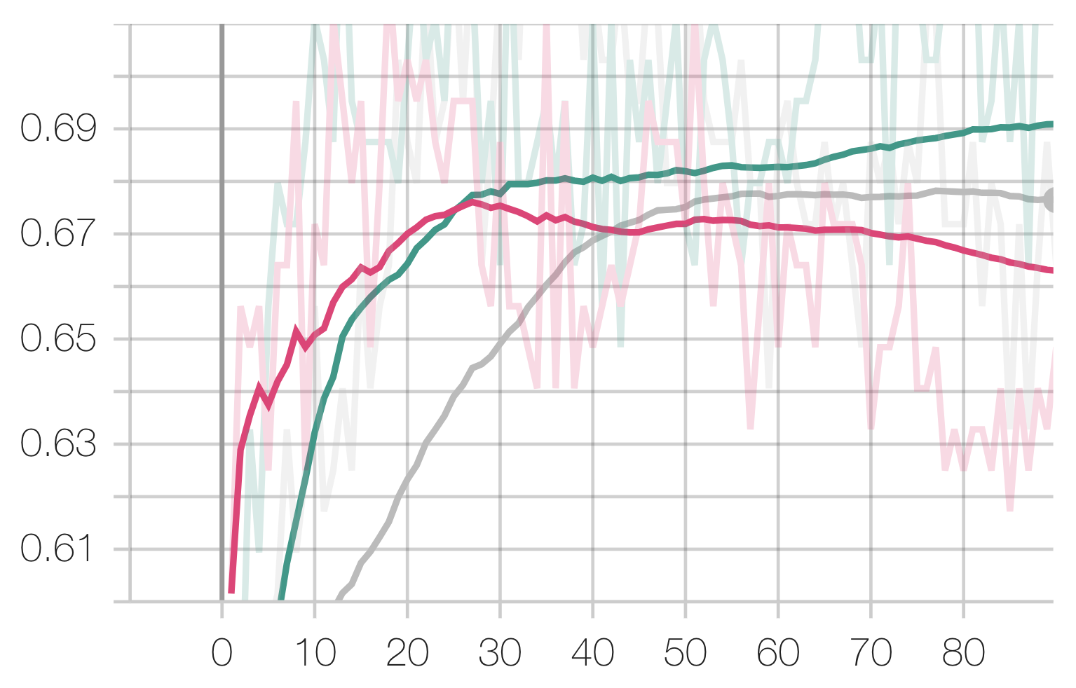
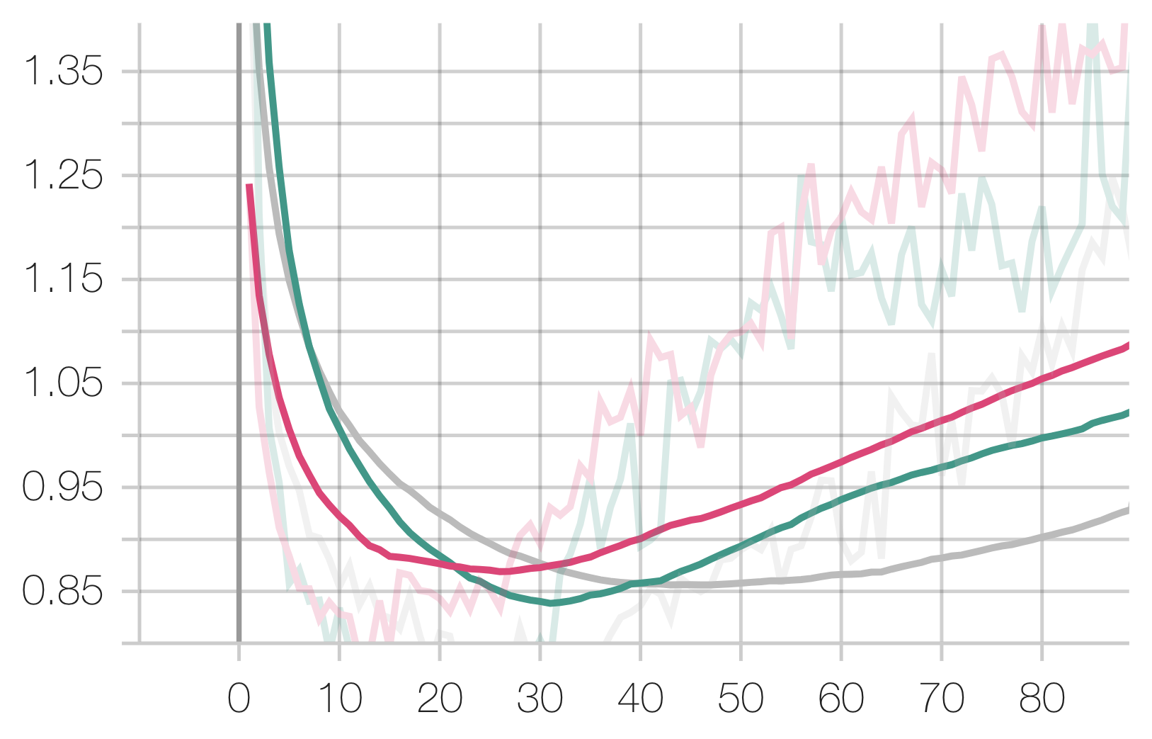
EEG Task:

Legend: Scratch, Speech, Radio, Audio

Radio Accuracy Curves (test split)

Radio Loss Curves (eval split)

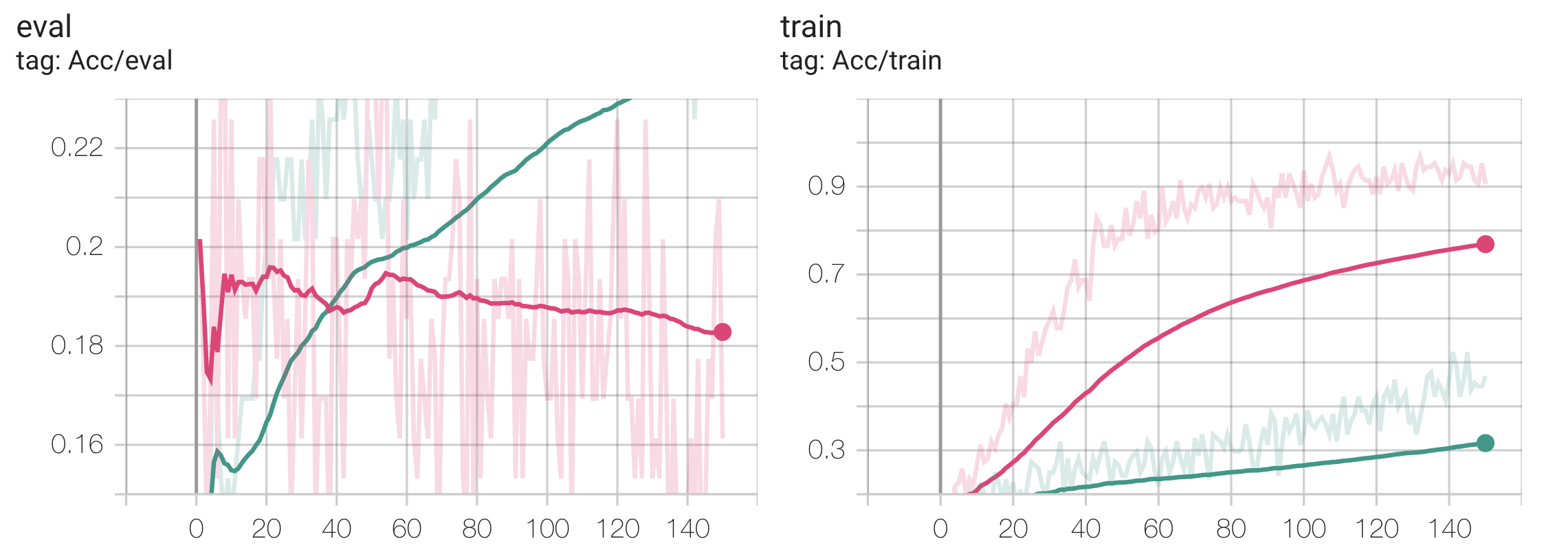
You may notice that performance hit a plateau very early, with all configurations reaching similar levels of performance. This is an addition to the fact that the eval losses hit a local minimum (if at all) before increasing. This implies over-fitting, which is confirmed by our train vs eval loss curves:

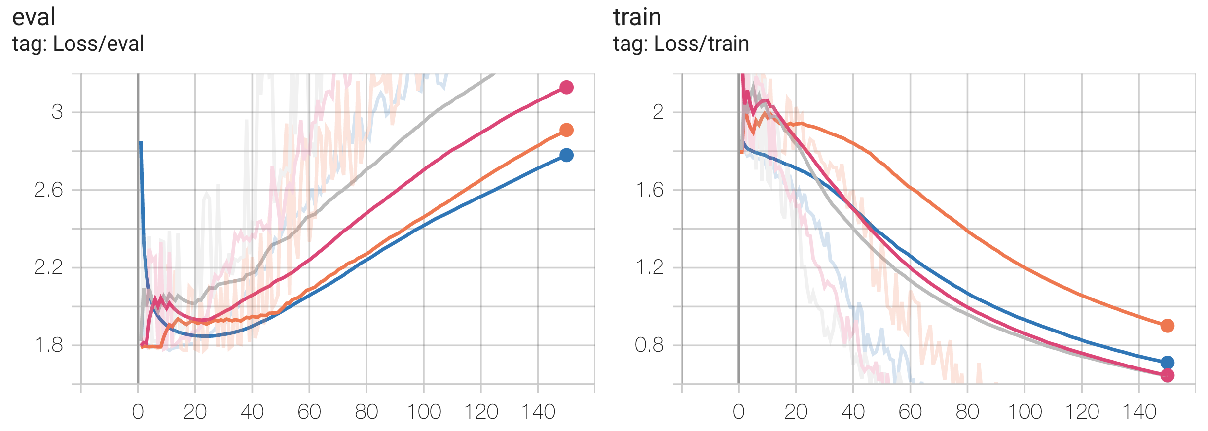
The first thing to note is that transferring from the Audio dataset (smallest) performed the best, whereas transferring from the Radio dataset (largest) performed the worst, which is unexpected. We posit this to be due to more significant task / data distributional differences between audio / digital signal and EEG signal, such that the pretrained knowledge had to be “unlearned,” and that the “knowledge” from the larger dataset was harder to “unlearn.”

However, this is not exactly conclusive either as this model did not demonstrate good generalization ability on EEG in the first place as it overfit very easily. In order to come to more conclusive results, future work has to be done to choose a less expressive model / better EEG dataset and re-run all these comparative experiments on them. We demonstrate that this is indeed the direction to proceed by showing that freezing many of the weights in the model (pretrained on Speech, because the Speech configuration performed similarly to the Scratch configuration) while fine-tuning on EEG actually results in better evaluation performance:

Pretrained on Speech, Transferred to EEG:

Legend: Freeze 60 Layers, No Freezing

10. References

Tingyan Kuang, Huichao Chen, Lu Han, Rong He, Wei Wang, and Guoru Ding. Abnormal signal recognition with time-frequency spectrogram: A deep learning approach, 2022. URL https: //arxiv.org/abs/2205.15001.
Wenhan Zhang, Mingjie Feng, Marwan Krunz, and Amir Hossein Yazdani Abyaneh. Signal detection and classification in shared spectrum: A deep learning approach. In IEEE INFOCOM 2021 - IEEE Conference on Computer Communications, pages 1–10, 2021. doi: 10.1109/INFOCOM42981. 2021.9488834.
Yuan Gong, Cheng-I Jeff Lai, Yu-An Chung, and James Glass. Ssast: Self-supervised audio spectrogram transformer, 2021. URL https://arxiv.org/abs/2110.09784.
J. Salamon, C. Jacoby, and J. P. Bello. A dataset and taxonomy for urban sound research. In 22nd ACM International Conference on Multimedia (ACM-MM’14), pages 1041–1044, Orlando, FL, USA, Nov. 2014.
Stefan Scholl. Classification of radio signals and hf transmission modes with deep learning, 2019. URL https://arxiv.org/abs/1906.04459.
Sören Becker, Marcel Ackermann, Sebastian Lapuschkin, Klaus-Robert Müller, and Wojciech Samek. Interpreting and explaining deep neural networks for classification of audio signals. CoRR, abs/1807.03418, 2018.
Kaggle Kaggle. Grasp-and-lift eeg detection, 2015. URL https://www.kaggle.com/ competitions/grasp-and-lift-eeg-detection/data.
Daniel S. Park, William Chan, Yu Zhang, Chung-Cheng Chiu, Barret Zoph, Ekin D. Cubuk, and Quoc V. Le. SpecAugment: A simple data augmentation method for automatic speech recognition. In Interspeech 2019. ISCA, sep 2019. doi: 10.21437/interspeech.2019-2680. URL https: //doi.org/10.21437%2Finterspeech.2019-2680.
Mingxing Tan and Quoc V. Le. Efficientnet: Rethinking model scaling for convolutional neural networks. 2019. doi: 10.48550/ARXIV.1905.11946. URL https://arxiv.org/abs/1905. 11946.

Multitask Learning Across Time-Series Spectrogram Tasks

Contents